Examining the Phillips Curve
1 Introduction
The inverse relationship between unemployment and inflation, described by the well known Phillips Curve, may not be as straightforward nor as stable through time as once proposed. On the other hand, the Phillips Curve may require more extreme ranges in unemployment and inflation in order to “come to life”. Rather, for periods of very tight labor markets and extremely high inflation, we tend to see a drastic difference in the strength of the inverse relationship between the two variables. This might lead one to postulate that there are, in fact, two relationships in play. The first relationship may correspond to periods of very tight labor markets (and very high inflation), and the second relationship may correspond to periods of relatively less extreme/tight labor markets and (often, but not always) relatively tamer inflation. Some have reasoned that the data should be modeled to include a “kink” wherein the relationship changes at some unemployment threshold. Others, including the original Phillips Curve model, might utilize a nonlinear term, or attempt various polynomial (e.g. quadratic, cubic) parametric approaches. In the following analysis, one can examine the results of a simple Bayesian “kinked” regression model and a Bayesian formulation of the original Phillips Curve model. Cubic and quadratic Bayesian regression models were also explored, but suffer too heavily from their parametric assumptions. The cubic and quadratic models are discussed and explored in more detail within the appendix.
It is important to note that one can find long periods where the Phillips Curve relationship flattens or even reverses. However, the investigation below desires to answer a different question (1) : how does the Phillips Curve differ from periods with tight labor markets versus periods of loose labor markets, and can we estimate where this threshold might exist? This problem is made more complicated by noting that there are only a few periods of extremely high inflation (or very tight labor markets). A preemptive critique might include having too few data points to make any conclusive arguments. While one should absolutely take into account that no context is truly the same throughout different periods in time, one might still formulate an informed prior for future contexts wherein we see very tight labor markets. Rather, one could think of the results of this analysis as a meta-prior on future data we have not yet seen. This approach, presumably, is better than doing nothing due to having too little data.
Then, a second (2) question revolves around which specification might better fit the data. While the kinked regression provides a distinct inference that curve models can’t quite provide (although, one can still find curve vertices), another question might center around which model “fits” the data better as a whole. Again, and as a point of caution, one should note that a model that “fits” the data better isn’t necessarily the model that will predict better in the future. On the other hand, and as a point of past inference, we can explore how these competing models compare relative to model fit throughout time.
Third (3), we wish to include inflation expectations within our explored models. In combination with the labor market “threshold”, we want to know if periods with very tight labor markets coincide with stable or volatile inflation expectations.
Fourth (4), and in a similar vain, we wish to investigate how, or if, supply shocks tie in to the above dynamic.
Last (5), the reader might be wondering about the path of inflation and unemployment simultaneously through time. For this, we can explore a Bayesian Structural Time Varying Vector Autoregressive (TV-VAR) model in the form of a Dynamic Linear Model. In doing so, we can then plot a three dimensional graph of the estimated joint contemporaneous evolution of inflation and unemployment through time against the true data.
2 Data
Data used in this analysis comes from the Federal Reserve Bank of St. Louis database, i.e. the FRED, from the Bureau of Labor Statistics, and from link (Petrosky-Nadeau and Zhang 2021). For inflation, the FRED series ID is “PCEPILFE” (link) is described as “Personal Consumption Expenditures Excluding Food and Energy (Chain-Type Price Index), Index 2017=100, Seasonally Adjusted, Monthly Frequency”. Then, the analysis below takes the annual percent change of PCEPILFE. Then, for “labor market slack” the data is cut into two periods due to availability of data. For the second period from 2000-12-01 to today the data consists of the series ID “JTS000000000000000JOL” from the JOLTS (Job Openings and Labor Turnover Survey, conducted by the BLS) divided by the series ID “CLF16OV” from the FRED. JTS000000000000000JOL is the “All areas - Job openings - Total nonfarm - Level - In Thousands - Seasonally Adjusted - All size classes - Total US”, and where CLF16OV is the “Civilian Labor Force Level, Thousands of Persons, Seasonally Adjusted” level. Finally, for the first portion of “labor market slack” the data consists of the vacancy rate from Petrosky-Nadea and Zhang (call it \(vr_{PNZ,t}\)) multiplied by the first entry in the second portion of “labor market slack” (call it \(JOLTS/FRED_{1}\)) divided by the last entry in PNZ, rather \(vr_{PNZ,T}\). In sum, the first portion of the labor market slack data consists of \(vr_{PNZ,t}*\frac{JOLTS/FRED_{1}}{vr_{PNZ,T}}\) for each \(t\).
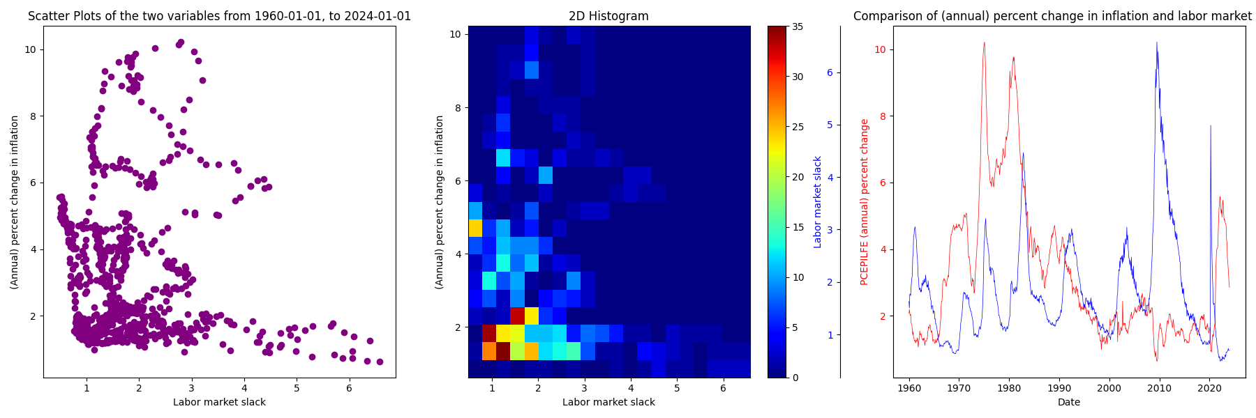
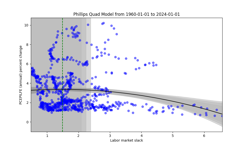
Below, there is some basic exploration of the data as a whole from 1960-01-01 to 2024-01-01.
3 Modelling approach 1: kinked Bayesian regression
Here, the basic modelling idea is to presume there is some “kink” point in the regression where the slope changes. One can place zero mean normal priors on the slopes on either side of the kink, alongside a uniform prior on the kink location (i.e., place a uniform prior on the starting point from the minimum unemployment rate ending at the maximum unemployment rate for the data under use within the regression). The mathematical details of the model are presented in the appendix.

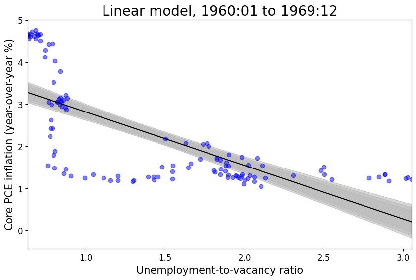
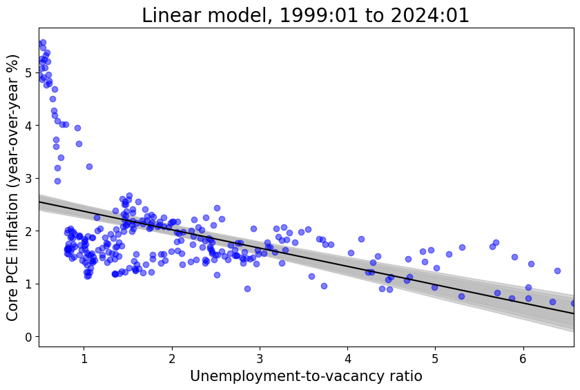
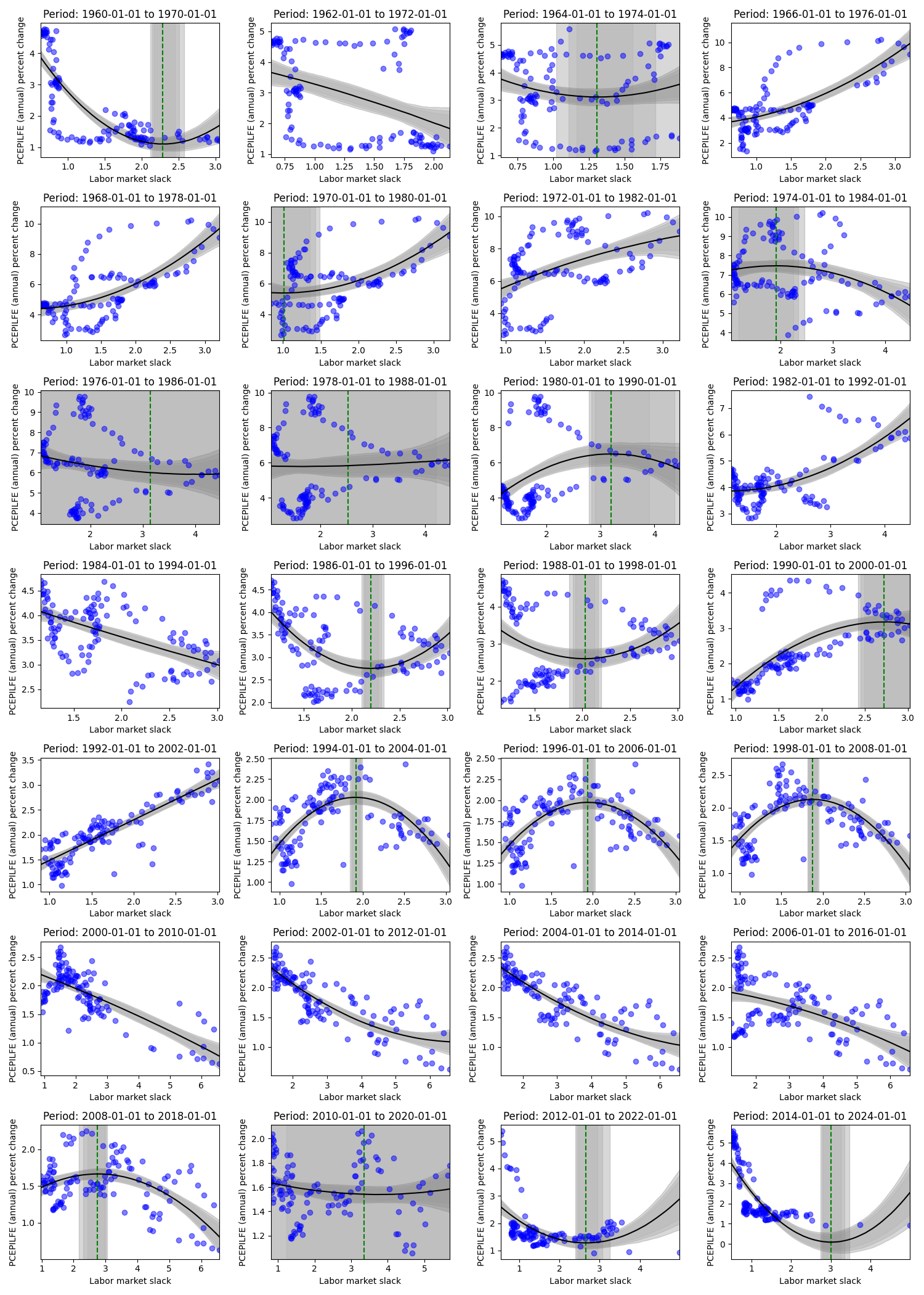
In the overall data, we don’t see a strong Phillips-like relationship. Next, let’s examine what the data looks like for 10 years by intervals of 2 years.

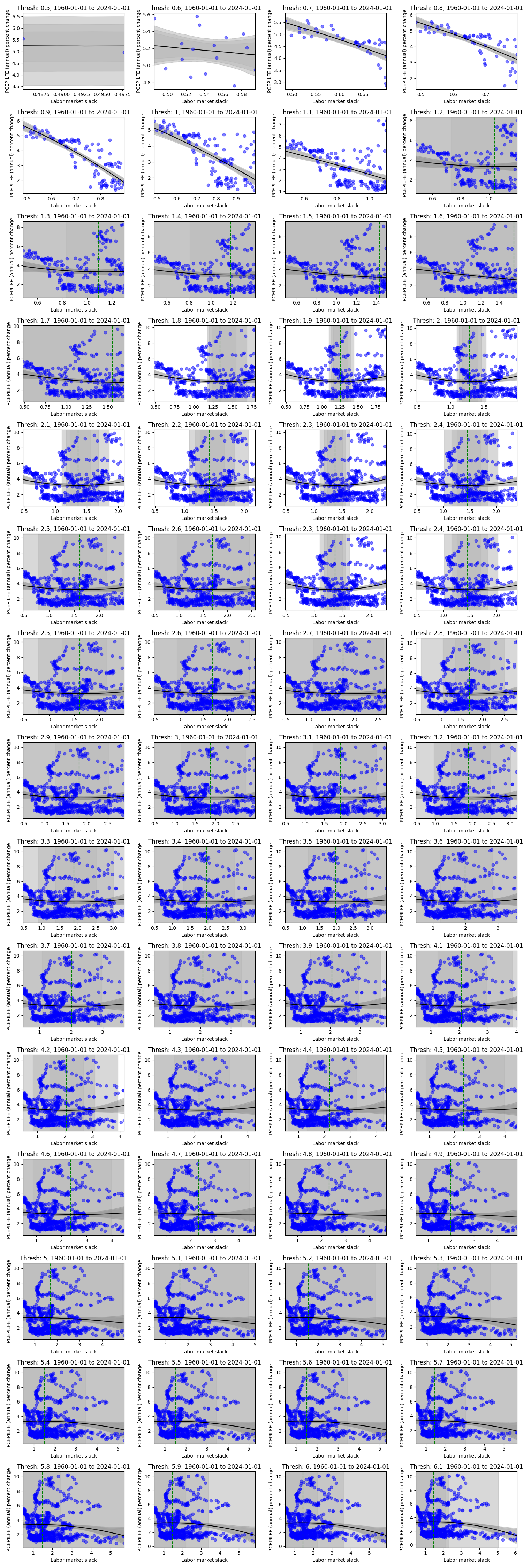
Looking at the figure above, we paint a fairly different picture (at different periods) than the first “overall” figure from 1960-01-01 to 2024-01-01. We can see flat and reversed relationships, and we can see how the estimated kink varies in location and uncertainty. In general, one might be quite wary of believing there is a stable Phillips Curve relationship both at the aggregate and the subperiod levels. However, let’s hone in on the data where the labor market slack is below a certain threshold, and let’s vary that threshold. To be clear, this means we are now combining data from different periods in time that meet this constraint.
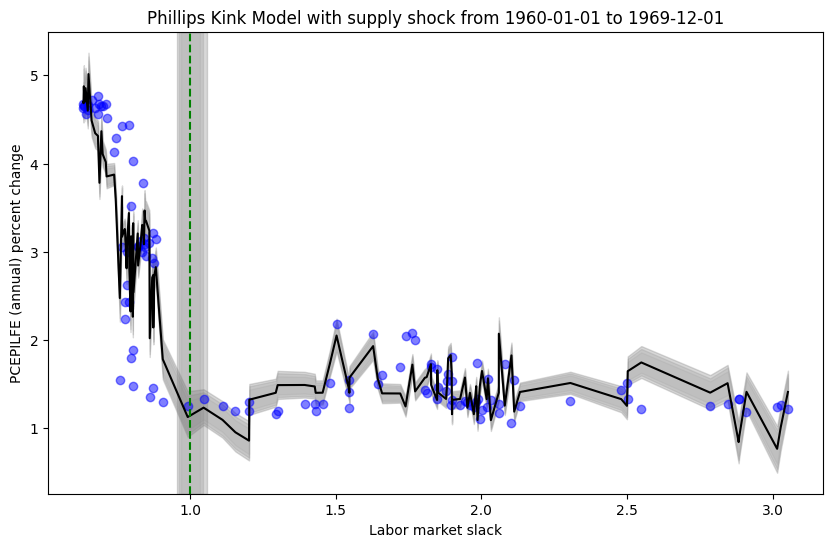
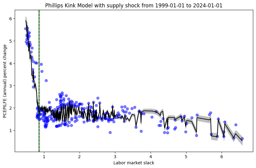
The data may be small for lower thresholds of labor market slack, but this downward slope to a kink somewhere at, or above .8, and below 1 seems to persist for all labor market slack thresholds (except for threshold 5.2, 5.9, and above 6 - which recovers the aggregate graph). Meaning, if we looked at this relationship in a vacuum without paying any attention to time, we would be reasonably sure that a change in the labor market slack - below this kink (somewhere around .8) - would imply a more drastic change in the annual percent change in inflation relative to a change in the labor market slack above said kink. Then, take note of the kinks in the figures above for data between 1960 - 1970, 2012 - 2022, 2014 - 2024, where again, we see a kink at, or around, .8 to 1. Rather, these periods at the beginning and end of the data set seem to drive the results below.
This may be a subtle (or obvious) point, but there are other periods of high inflation and relatively tight labor markets, but for the same labor market tightness, there are other periods with much lower inflation. Rather, there are instances (a) of labor market slack slightly above 1 with high inflation, but there are also other (b) periods where inflation is relatively low at the same labor market slack. In turn, it seems these “other” (b) periods are more frequent than the (a) periods, and in turn (b) washes out what could have been evidence of kink like behavior from (a). However, for cases (c) where labor market slack is below 1, we tend to see only instance of high inflation with no cases (d) that would include low inflation and low labor market slack. Rather, there is no (d) to analogously wash out (c). Then, the results of the model are exactly what we would expect from examining the data.
It could be the case that (d) events will occur in the future, washing out our results driven from events (c), but this is yet to be the case, and so these results may serve as a prior in understanding the relationship between the two variables. Or, like the rest of the labor market thresholds, the relationship between labor market slack and inflation may become a wash, flattening out in the future.

Next, one can explore the original Phillips curve.
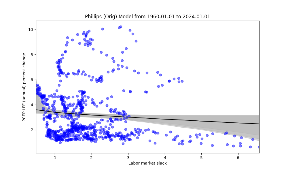
4 Modelling approach 2: Phillips (original)
The following results are using the model cited in (Benigno and Eggertsson 2023), where details are provided in the appendix. Roughly speaking, this model seems to behave more sensibly than either the quadratic or cubic models, and potentially better than the kink model. The downside to the curve model, as stated earlier, is the loss of the “kink” inference. We explore the data in a similar fashion, informed from the results of the kink model, however.
Similarly, we explore data of 10 years by intervals of 2 years, below

We see relatively similar fits. Next, we explore the “threshold” models, again to see if it aligns with the kink model.

We can many of the analogous takeaways seen in the kink model. While the kink does aid in the inference, we can still see a steeper slope roughly up to the .8-1 range in the labor market slack.
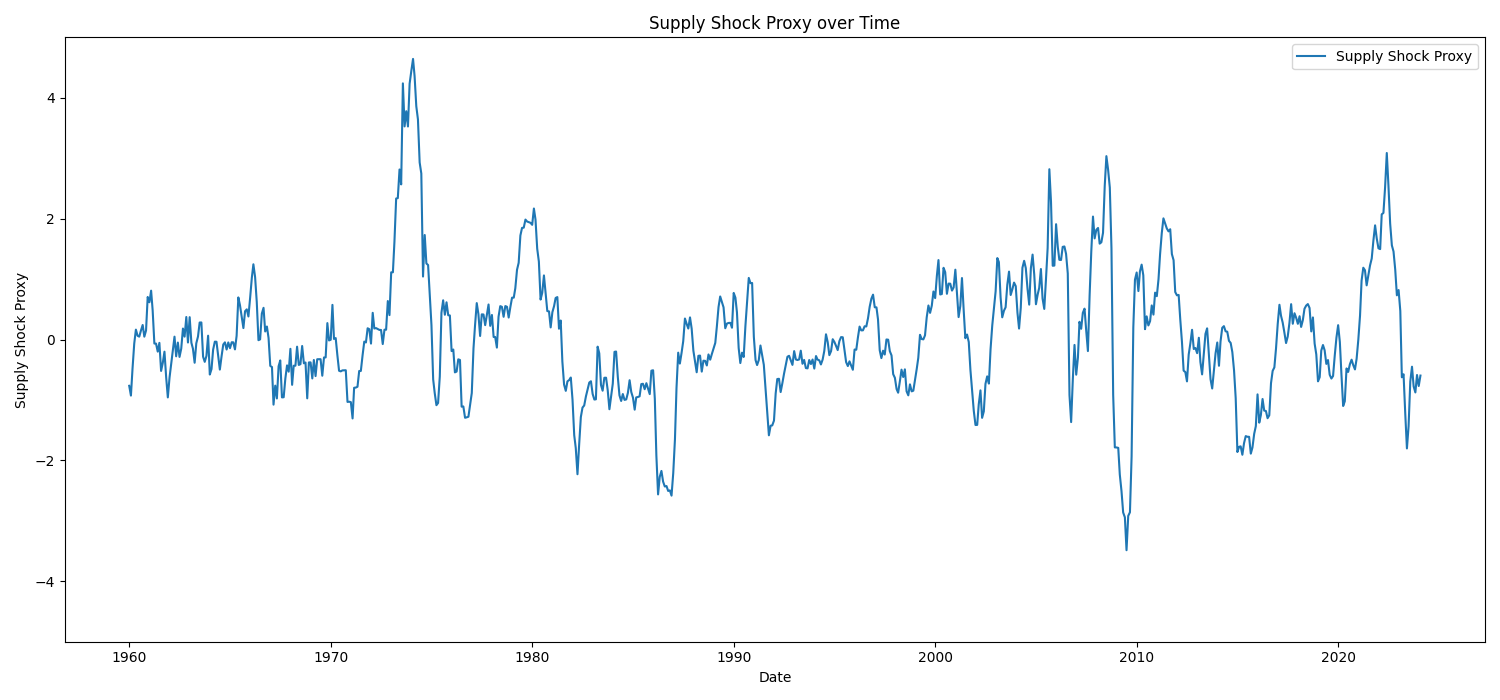
5 Supply shocks
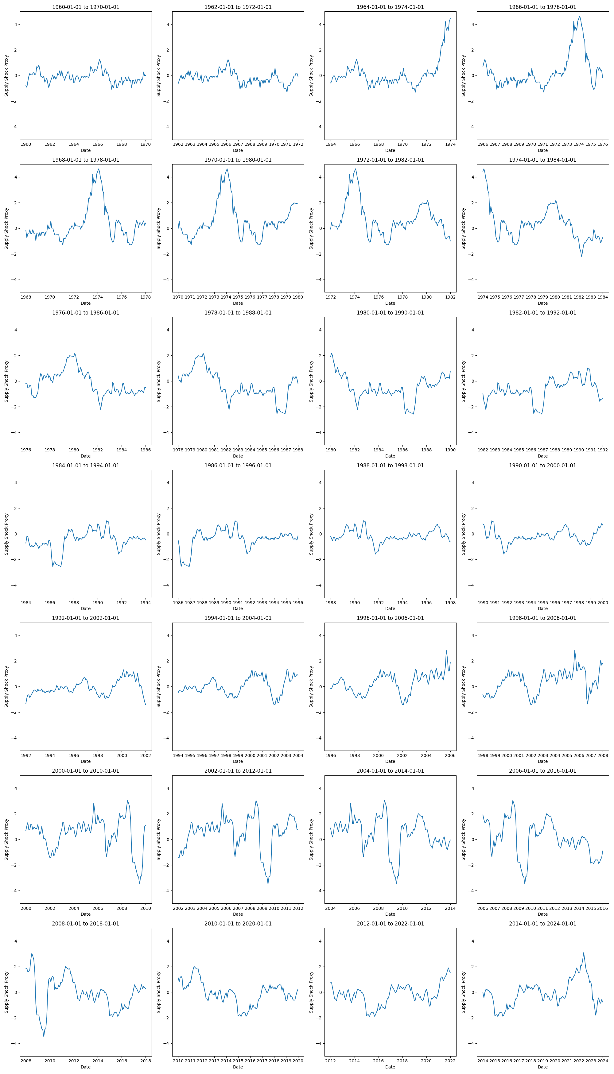
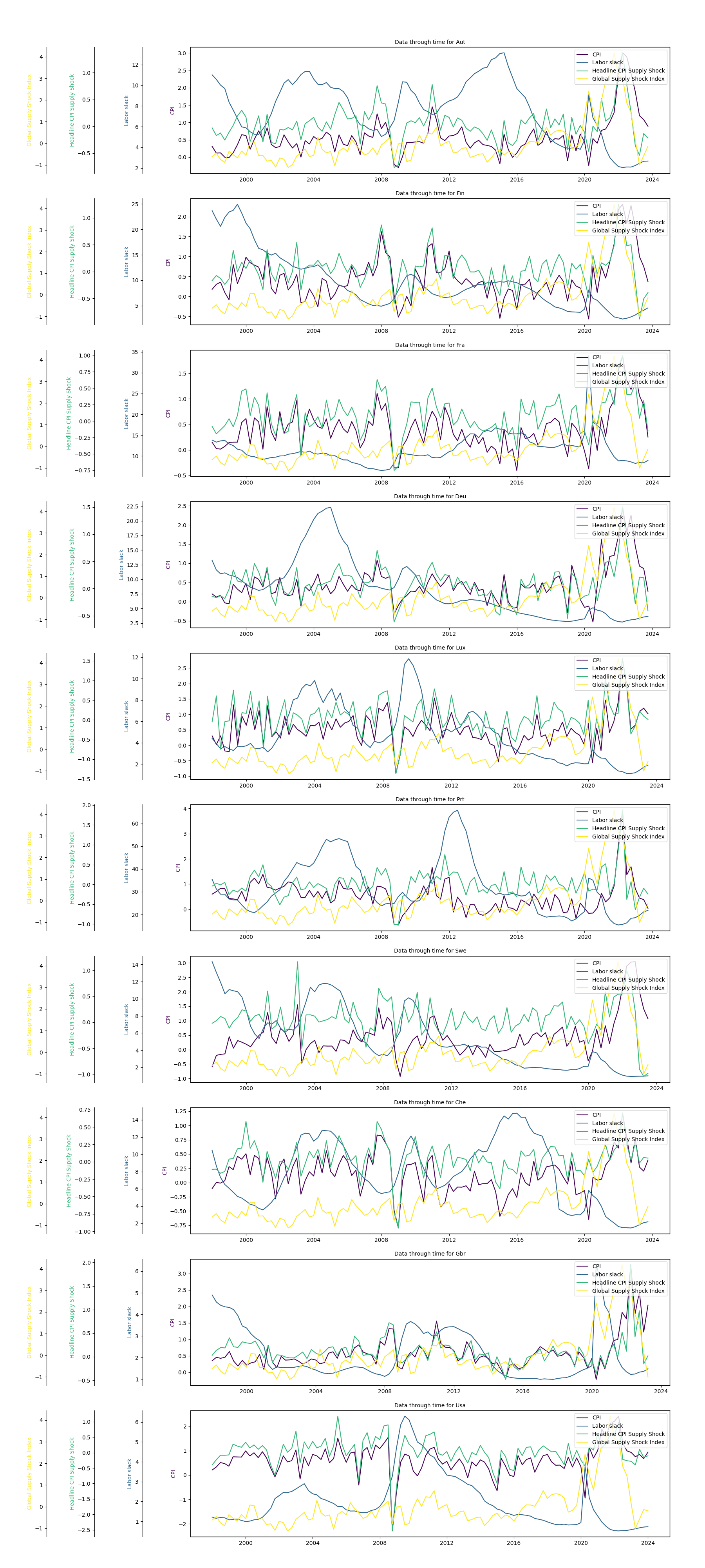
Below are supply shocks over the same 10 year periods in intervals of 2 years. To obtain this supply shock variable, take the annual percent change of CPIAUCSL minus the annual percent change from CPILFESL. On a first pass, we see shocks in the early to mid 1970s, around 1980, early 1980s, mid-late 1990s, maybe again around 2000, early 2000s, mid and late 2000s, with a large dip circa 2010 and large (excess) rebound early 2010s, followed by a dip in the mid 2000s and a large upward swing early-mid 2020s followed by a downward spike.
Then, it might be useful to use the following graphs as they are cut up into periods that match the models above. Perhaps the most noticeable aspect is the lack of supply shocks in the first two graphs. Note that the first graph in the kink models from 1960-01-01 to 1970-01-01 had a pronounced kink (with analogous graph from the original Phillips model). Then, for last two graphs we see more variation in the supply shocks in the first two graphs, but recall that these periods from 2012-01-01 to 2022-01-01 and 2014-01-01 to 2024-01-01 have pronounced kinks. Rather, the role of supply shocks on these strongly kinked periods seems potentially mixed as the earlier case includes minimal volatility in the supply shocks whereas the later case displays quite a bit more. It is hard to say from simple inspection.
6 Periods of relatively stable expected inflation, and conditioning on supply shocks
Below we examine the fitted model without the supply shock and with the supply shock for these two relatively stable periods of inflation expectations.
6.1 Model fits without supply shock
Kink model in relatively stable periods (without supply shock covariate)
Phillips (original) model in relatively stable periods (without supply shock covariate)
Phillips (linear) model in relatively stable periods (without supply shock covariate)
6.2 Model fits with supply shock
Next, we can see how the model behaves when including an additional covariate for supply shocks. Note that the graphs below display only the inflation and labor market slack axis, but each point corresponds to the observation supply shock used to fit the data.
Kink model in relatively stable periods (with supply shock covariate)
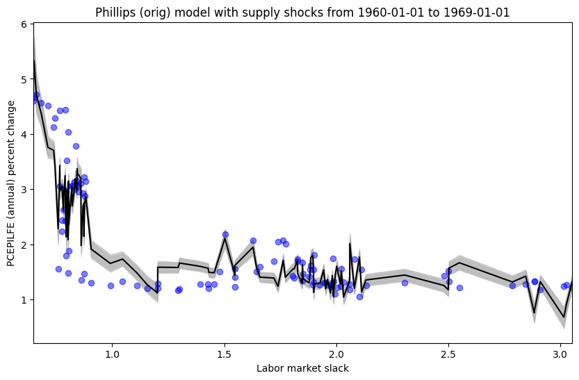
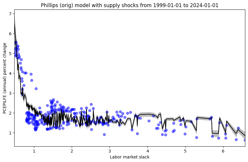
Phillips (orig) model in relatively stable periods (with supply shock covariate)
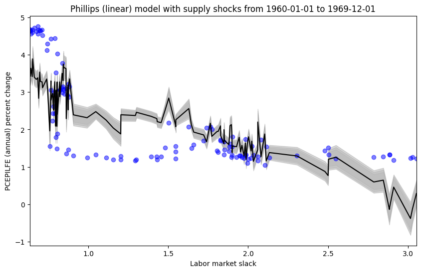
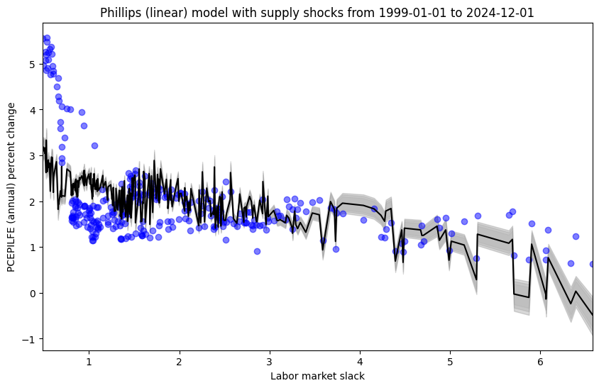
Phillips (linear) model in relatively stable periods (with supply shock covariate)
It seems that the addition of the supply shock variable explains more of the variation in inflation in all cases. Rather, if one were to calculate any performance or fit metric based on the distance between the model prediction and observed values, the model including the supply shock variable would dominate the model that does not include the supply shock variable.
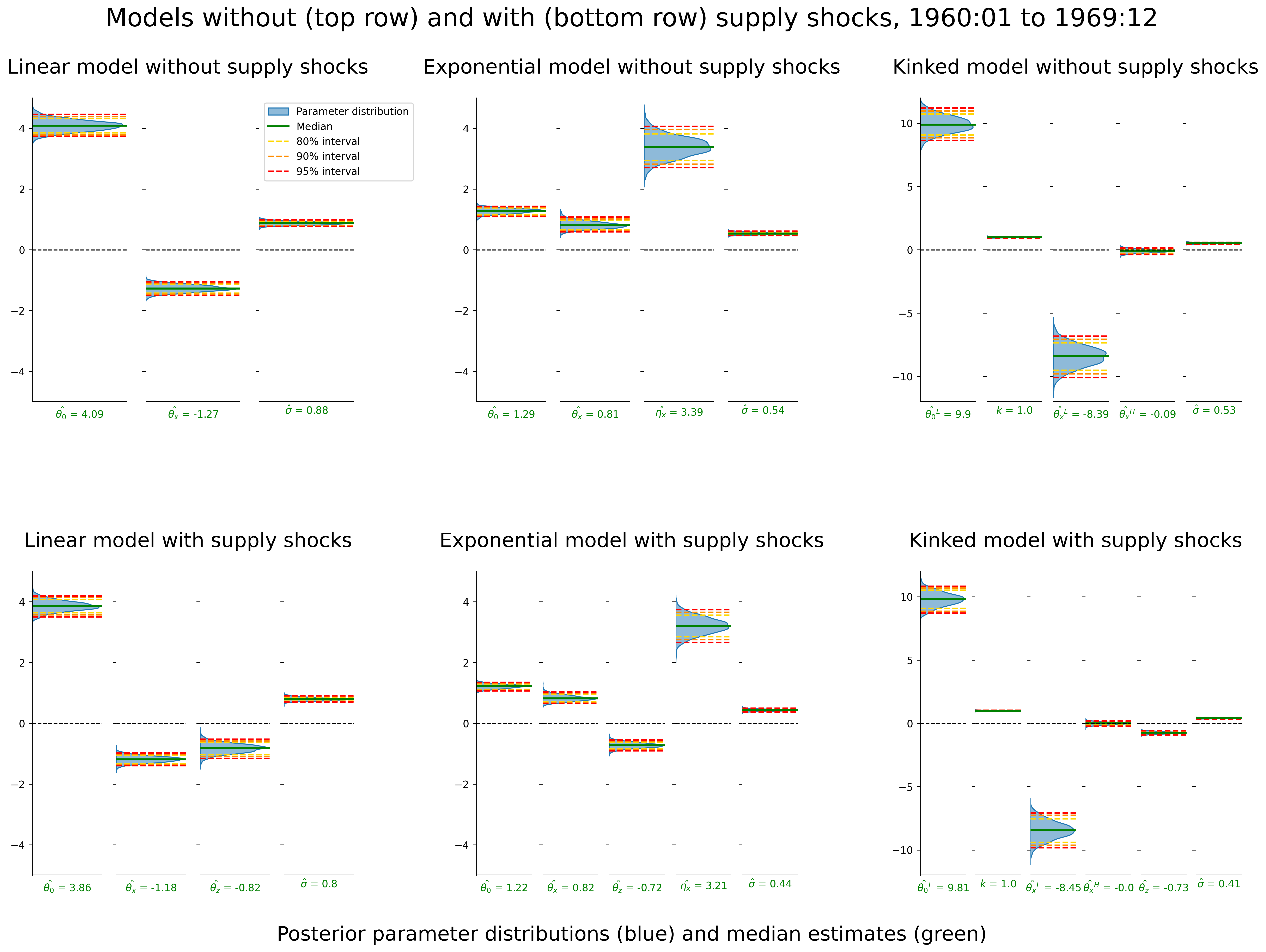
6.3 Posterior parameter estimates with and without supply shocks
On the other hand, we may ask whether the supply shock variable is “stealing” the story from labor market slack, or other parameters estimated in the model. Rather, are supply shocks behaving like an “omitted variable”? One can answer this question in a variety of manners. First, one can ask if the inclusion of the supply shock variable drastically changes the estimates of the other parameters. See the figures below to garner precise answers to this question. Supply shocks are not “corrupting” the story, but they are adding to the explanation. Rather, in each model type at each time period, we see that the inclusion of the supply shock variable reduces the estimate of observational noise - or, it explains more of the variation in the data. This should intuitively align with the plots provided in the previous section.

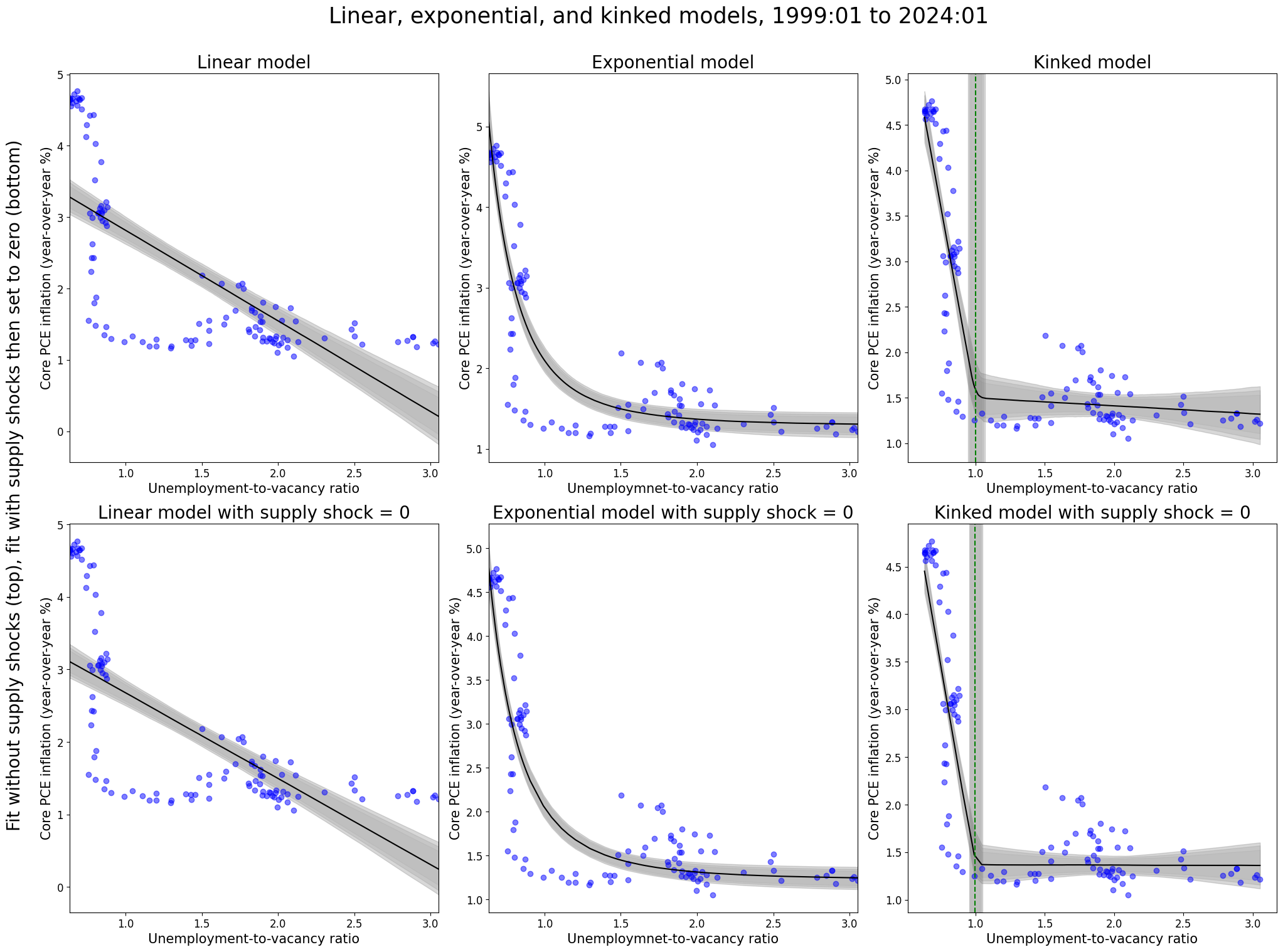
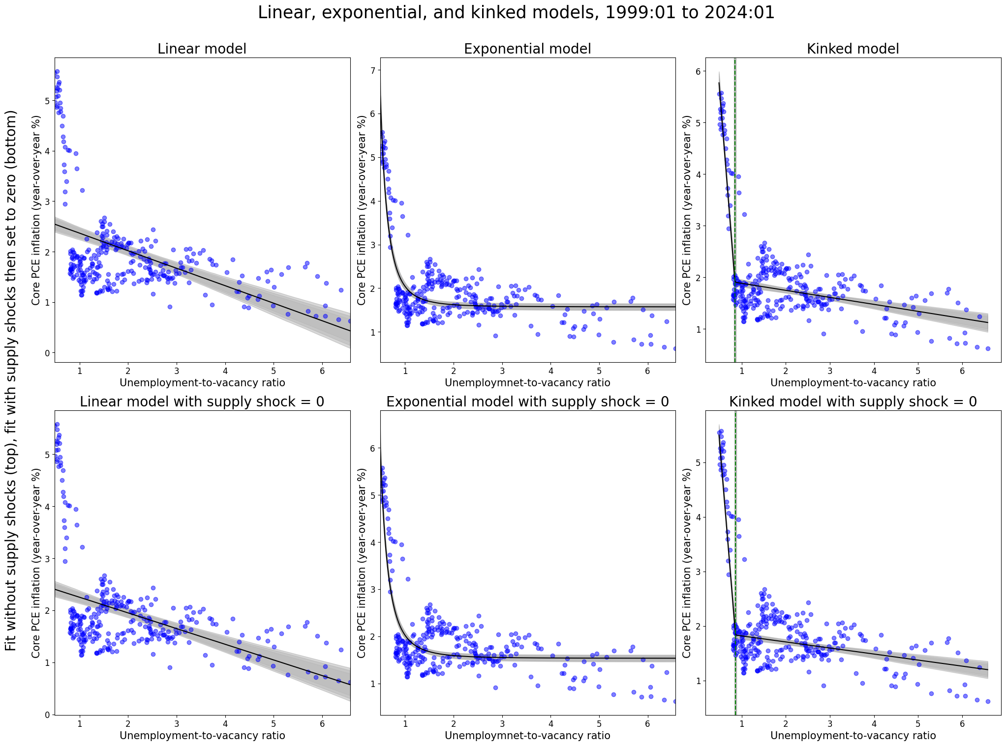
6.4 Fit without supply shock vs. fit with supply shock (and set to zero)
Next, one can fit the model without the supply shocks (top rows) and examine how the model fit compares to a model fit with the supply shocks. However, in the latter model type one can then set the supply shocks equal to zero (bottom rows). Just as the parameters in previous section did not drastically change after including the supply shock variable, the models below analogously display that fitting the model and including the supply shock does not drastically change the model fit. Rather, if including the supply shocks did “corrupt” the other parameters (and in turn the overall model), then we would expect to see a difference between the top rows and the bottom rows even with setting the supply shocks equal to zero. This is just another way to display the same conclusions drawn from the previous section.
6.5 Bayesian model comparison with supply shocks
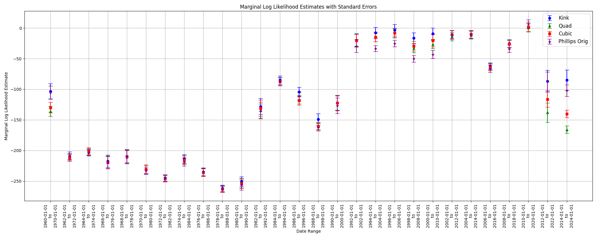
In the section below, I used ELPD (Expected Log Predictive Density). Further, these metrics were transformed to be in line with a log10 scale. While ELPD is quite interesting in it’s own right, this is not an approximation of marginal likelihood! See the following few sections for elaboration. This section will be updated in the future, but my initial guess is that relationships between the models will maintain the same ordering.
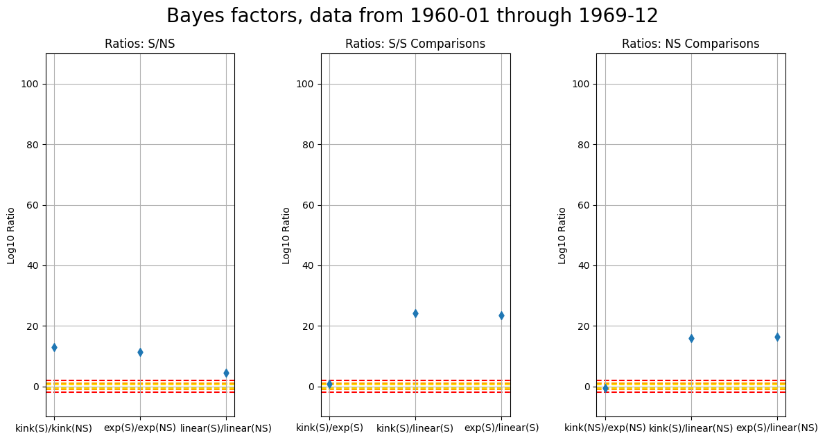
Below, a value of 2 decisively favors the model in the numerator. More details of Bayes factors and model comparison are in the next section. The following graphs emphasize that the inclusion of supply shocks always implies a decisively favored model over a fit that excludes the supply shock variable. This is true for both periods. Again, this corroborates the previous findings, but does not imply the labor market slack (and other model parameters) are incorrect as we previously discussed in the posterior parameter density plots above.
Then, we see that the kink model is favored at the “substantial” level (.78) for the period from 1960-01 through 1969-12 when including the supply shocks (S), and conversely that both dominate the linear model including the supply shocks. Then, it is of slight interest to note that without including the supply shocks (NS), we see the exponential model is favored at the “substantial” level (-.62) over the kink model.
Then, in the period from 1999-01 through 2024-01, we see the kink model is decisively favored over the linear and exponential models whether or not supply shocks were included.

6.6 Bayesian model comparison, Bayes Factor, ELPD
6.6.1 Bayes Factor, Marginal Likelihood
One can obtain the model marginal likelihood as
\[p(\mathbf{y}|Model) = \int p(\mathbf{y}|\boldsymbol{\theta},Model)p(\boldsymbol{\theta}|Model)d\boldsymbol{\theta}\]
where \(\boldsymbol{\theta}\) are the parameters corresponding to the \(Model\). Then, one can obtain evidence (\(K\)) a ratio of the posterior odds of \(Model_1\) and \(Model_2\) as follows
\[ \frac{p\left(Model_1 \mid \mathbf{y}\right)}{p\left(Model_2 \mid \mathbf{y}\right)}=\frac{p\left(Model_1\right)}{p\left(Model_2\right)} \frac{p\left(\mathbf{y} \mid Model_1\right)}{p\left(\mathbf{y} \mid Model_2\right)} \]
so that we have \(posterior \ odds = prior \ odds \ \times \ Bayes \ factor\). It is important to note that the marginal likelihood is integrating over the priors, and not the posterior \(\boldsymbol{\theta}\). Then, a note on penalizing complexity.
Recall that we have \(\underbrace{\frac{P\left(M_1 \mid D\right)}{P\left(M_2 \mid D\right)}}_{\text {posterior odds }}=\underbrace{\frac{P\left(D \mid M_1\right)}{P\left(D \mid M_2\right)}}_{\text {Bayes factor }} \underbrace{\frac{P\left(M_1\right)}{P\left(M_2\right)}}_{\text {prior odds }}\)
(also, if we have equal prior odds, then we have posterior odds = Bayes factor)
Basic (model is \(M\)): \(P(\) Data \(\mid M)=\int P(\) Data \(\mid \theta, M) P(\theta \mid M) d \theta\)
Example illustration: Then, let \(M_1\) be a model with parameter \(\theta\) that is discrete and takes on three values. Then we have
\[ P\left(\text { Data } \mid M_1\right)=P\left(\text { Data } \mid \theta_1, M_1\right) P\left(\theta_1 \mid M_1\right)+P\left(\text { Data } \mid \theta_2, M_1\right) P\left(\theta_2 \mid M_1\right)+ P(Data|\theta_3,M_1)P(\theta_3|M_1) \]
versus a model \(M_2\) that has discrete parameter \(\eta\) that has two values. Then we have
\[ P\left(\text { Data } \mid M_2\right)=P\left(\text { Data } \mid \eta_1, M_2\right) P\left(\eta_1 \mid M_2\right)+P\left(\text { Data } \mid \eta_2, M_2\right) P\left(\eta_2 \mid M_2\right) \]
Then, if \(\theta_{1:3}\) or a sub portion do not explain the data well, then \(P(Data|M_1)\) can be diluted. Then, one can extrapolate to not just having more discrete values, but also more parameters in general. If you include a bunch parameters that do nothing in terms of explaining the data, they will dilute the Bayes factor.
\[ \ln (p(Data \mid \theta, M))=\ln (\widehat{L})-\frac{n}{2}(\theta-\hat{\theta})^{\mathrm{T}} \mathcal{I}(\theta)(\theta-\hat{\theta})+R(x, \theta) \]
\[ p(Data \mid M) \approx \hat{L}\left(\frac{2 \pi}{n}\right)^{\frac{k}{2}}|\mathcal{I}(\hat{\theta})|^{-\frac{1}{3}} \pi(\hat{\theta}) \]
\[ p(Data \mid M)=\exp \left(\ln \widehat{L}-\frac{k}{2} \ln (n)+O(1)\right)=\exp \left(-\frac{\mathrm{BIC}}{2}+O(1)\right) \]
The marginal likelihood is often intractable (particularly in high dimensional models), so sampling methods are often used. From my understanding, MC sampling/integration can be inefficient if \(p(\mathbf{y}|\boldsymbol{\theta})\) is very small for most prior samples (often the case). Then, it seems like there are alternative approaches that use MCMC to sample from the posterior distribution - focusing on high likelihood regions of the parameter space - then use these samples to estimate the marginal likelihood using techniques like the Harmonic Mean Estimator or Bridge Sampling. To my understanding these MCMC samples are used in an importance sampling schema to recover the marginal likelihood which by definition is not conditioned on the posterior \(\boldsymbol{\theta}\).
For a very nice treatment of marginal likelihoods see (Gamerman and Lopes 2006), Chapter 7 Further topics in MCMC. Of note, MC approximations were argued to work poorly and are unstable in cases of disagreement between prior and likelihood (Raftery and Lewis 1996). The alternative is to use importance sampling, where the importance density is often chosen to be the posterior density. There are various proposal density approaches, and a comparison of several estimators are provided by (Lopes and West 2003). It is likely our study will either use Bridge Sampling or Harmonic Mean.
Then, moving a step forward, we have the Expected Log Predictive Density, or ELPD. This metric, unlike the marginal likelihood, integrates over the posterior \(\boldsymbol{\theta}\), obtaining the posterior predictive distribution, which is then used in finding the expectation of the log predictive density over all possible future data. Of course, we do not know what the future data is, so leave-one-out cross validation is used as a proxy. However, note that the posterior \(\boldsymbol{\theta}\) have already updated on all the data, so the leave-one-out cross validation is slightly tainted (perhaps the more appropriate approach would be to obtain posterior \(\boldsymbol{\theta}_{-y_i}\), integrated out to get the posterior predictive to then use in the LOO-CV approach, but this, of course, would be extremely expensive). A nice development of both Bayes Factor and ELPD is provided by (Bruno Nicenboim and Vasishth). The author also notes that the optimistic results of posterior predictive checks suffers from the same concept mentioned above, but is still a nice tool for checking gross model misspecification.
Note that in the analysis here the marginal likelihood is approximated as the Pareto-smoothed importance sampling leave-one-out cross-validation (PSIS-LOO-CV) giving the expected log pointwise predictive dendsity (elpd). Standard errors are also estimated. The metric also provides diagnostic warnings. Details (Vehtari, Gelman, and Gabry 2016). Note that the ratio of ELPD is not the same as the criterion for the Bayes Factor. However, we can intuit that that an ELPD larger than (several) standard errors of another model provides evidence of a favored model. One hand-waving way to analogize the difference from the Marginal Likelihood to the ELPD might be to think of the Marginal Likelihood as being closer to a “prior predictive check” in flavor, whereas the ELPD may be closer to a “posterior predictive check” in essence.
EDIT: below uses ELPD…
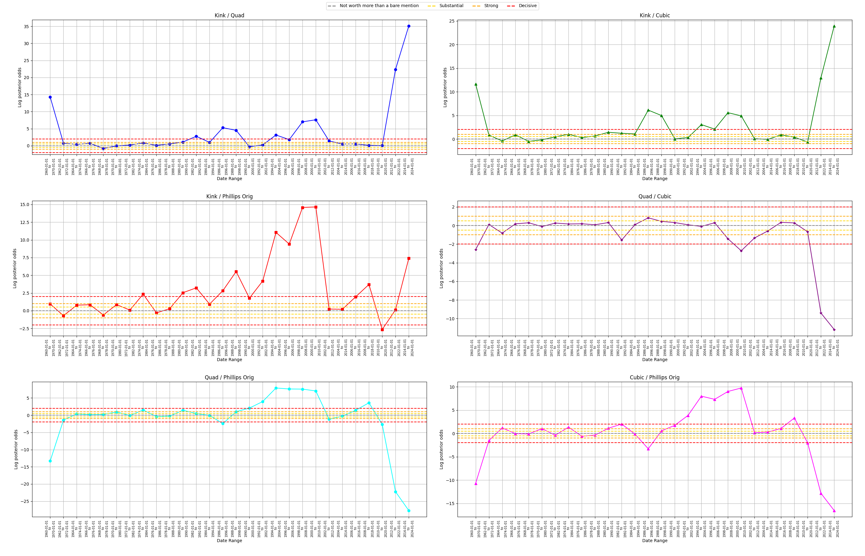
We can then examine the posterior odds in a pairwise fashion below. In fact, if we have equal priors on each model, then these graphs are equivalent to Bayes factor for each pairwise comparison. Then using the nomenclature from (Kass and Raftery 1995) one can see evidence of differences between the models at “Not worth more than a bare mention”, “Substantial”, “Strong”, and “Decisive” levels.
A few notes regarding the figure below:
The kink model dominates the quadratic and cubic models
The kink model largely dominates the original Phillips model except for the period from 2010-01-01 to 2020-01-01
Of note, the kink and original Phillips models trade wins earlier on, however, in the period of distinct kink-like behavior in 1960-01-01 through 1970-01-01, we see “Strong” evidence in favor of the kink model over the original Phillips model. Similarly, we see the kink model dominate in the very kink-like period of 2014-01-01 through 2024-01-01
It is of note that the kink model does “Decisively” lose relative to the original Phillips model in one period from 2010-01-01 through 2020-01-01. Of note, the kink model is flat but finds it’s kink to the right of labor market slack at value 5, but the original Phillips model has a steep curve for low labor market slack values followed by a flat line. Then, note that this is the only kink found at a higher labor market slack value. Rather, if one is using the kink model and finds a kink in the data with high labor market slack, one might seek to use a different model as this is likely not trustworthy. On the other hand, we can see that the parametric nature of the original Phillips curve enforces an earlier dramatic curve, and fits the data better for these rare instances where the kink model estimates a kink at higher labor market slack values
The cubic model seems to dominate the the quadratic model, particularly for the last periods
The quadratic model dominated the original Phillips model in the periods roughly from 1992 through 2010. Then the original Phillips model dominates the quadratic model elsewhere
This aligns with our earlier intuitions. Note the kink model dominates the quadratic model for the same periods. Rather, the quadratic model cannot capture these kinks of which the original Phillips model and the kink model “find”. On the other hand, the kink model does not get dominated by the quadratic model in any period. Note in the appendix, the quadratic model does fit the data quite well for the periods 1992 through 2018, and in particular, picks up on the concave quadratic behaving data circa 1994-2008 - data the original Phillips model cannot quite capture. The kink model, however, is able to capture this data, indeed fitting it even better than the quadratic model
Then, by a transitive extension of the argument above, for this reason the kink model dominates the original Phillips model in the period from 1994 through 2010
Statements regarding the quadratic and original Phillips model can analogously be applied to the relationship between the cubic model and the original Phillips model
NEXT STEPS: obtain marginal likelihoods for models using bridge sampling or harmonic mean for the models already developed. Do the same for the Gaussian Process below. Obtain the ELPD for the Gaussian Process below (harder said than done…).
- [Edit: I believe I have the marginal likelihood for the GP, now need to get ELPD for GP and marginal likelihoods for original models]. Although, it seems like the log marginal likelihood of a single point, or rather the sum of the marginal likelihood points divided by the number of training points…investigating
- [Edit: I believe I have the ELPD for the GP, the value makes sense, slightly better than ELPD for other models, but there is a very slight potential extra step I have to do. Also, I think I can compute SE for the ELPD… remaining task is marginal likelihood for original models].
- For the marginal likelihood of the original numpyro models, there seems to be no marginal likelihood tools (i.e. bridge sampling or exact calculations - it seems we could do exact calculations in the GP case), and so it looks like I may need to figure out how to get R’s bridge sampling package running in Python…
- Bridge sampling to get the marginal likelihoods is not easy… but with a dummy example I was able to get the marginal likelihood from a more custom bridge sampling from my numpyro model in python (adapted code from online), and then compare it to the marginal likelihood using the numpyro samples –> sent to R –> to then be used with the bridgesampling package in R (there is no bridgesampler package for python). The marginal likelihoodds match. So, hopefully I can now get the marginal likelihoods (via python implementation of bridge sampling) for the original models…
- Starting to get marginal likelihoods, and we see that kink > exp > quad > linear as we might hope. Still need to dig around the exact marginal likelihood of the GP as it seems like it is only of one point (or it is the average of the points… i.e. maybe just mutiply by N) <– this was correct, digging in the source code, they are scaling (dividing by N), now its clear GP > kink > exp > quad > linear for the marginal likelihood. For ELPD we see the same (I believe, checking)
- Summarizing,
- for the Non GP models:
- we have Marginal Log Lilikelihoods (mll) through bridge sampling. The code for the bridge sampling was tested using a dummy example against using the same in R where there is a package for bridge sampling (there is no bridge sampling package in python).
- we have the ELPD via Arviz package in python
- for the GP model:
- we have the exact mll via GPyTorch
- we built a custom ELPD via CV-LOO of the predictive distribution (checking if actually predictive distribution or something slightly different. score seems in line, however, with what we would expect relative to the other models). I believe we can get the SE for the ELPD just as in Arviz…
- for the Non GP models:
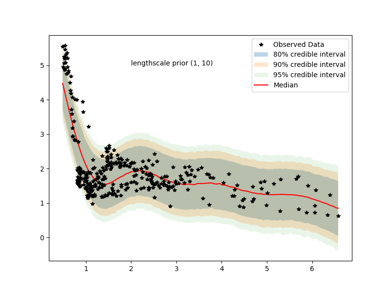
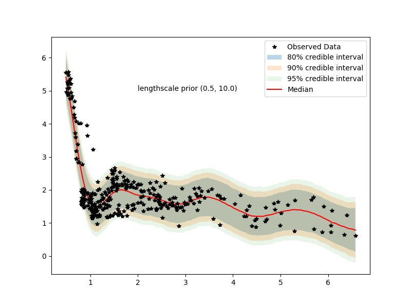
7 Modelling approach 3: Gaussian Process Regression (HMC)
The approaches above are all parametric. However, we would like to compare these models to a nonparametric approach such as a Gaussian Process. For details regarding Gaussian Processes, please see G: Gaussian Process Math (priors on hyperparameters + HMC).
Of particular note, most Gaussian Processes estimate the hyperparameters via MLE, MAP, or other optimization techniques. However, in doing so, the posterior predictive will inherently underestimate uncertainty. In general, obtaining the posterior distributions for the hyperparameters is not an analytic (conjugate) task, nor is it typically easy to set up conditionally conjugate distributions and utilize Gibbs sampling. Rather, MCMC approaches are typically preferred for this setting. In our case, we use the NUTS (HMC) algorithm. Then, since we can obtain the samples of the posterior hyperparameters, we can integrate the hyperparameters out of the model to obtain a truly posterior predictive distribution.
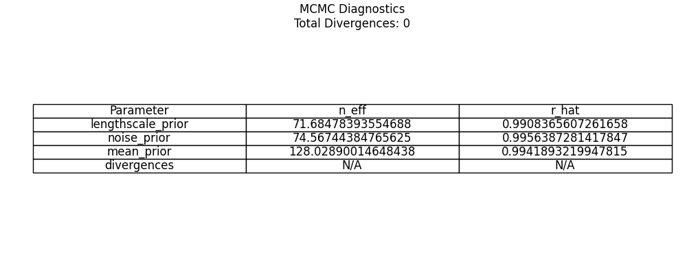
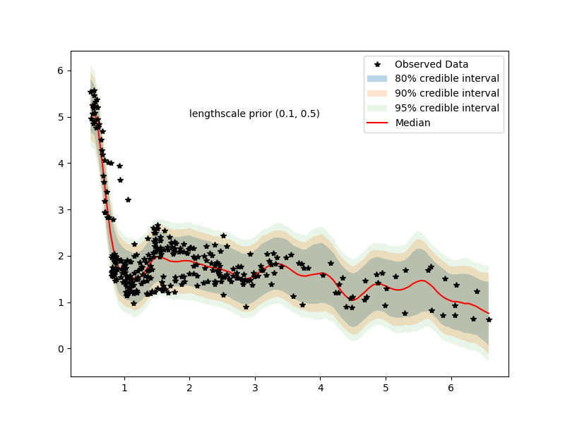
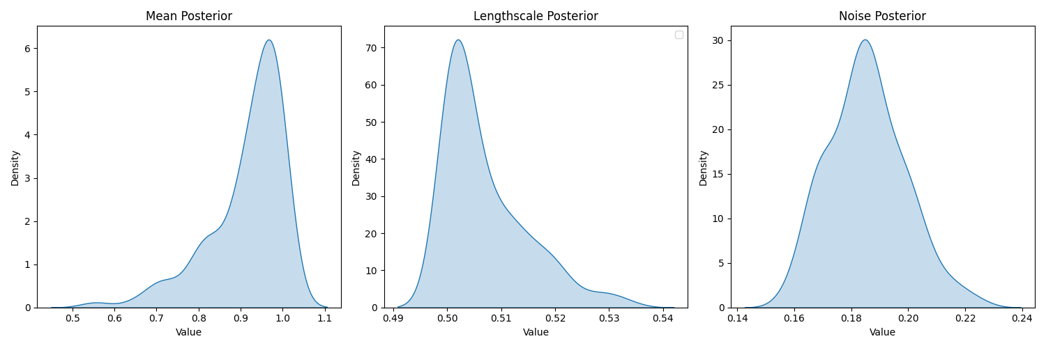
Our model uses a standard RBF kernel with priors on the observation noise, lengthscale, mean. Below, I provide examples of the output for the Gaussian Process approach. In the first column, I provide a model with 10 warm-up samples and 10-samples. We can see by the posterior predictive and the diagnostics that this model may require more samples. On the right, we increase the warm-up to 100 and samples to 100.
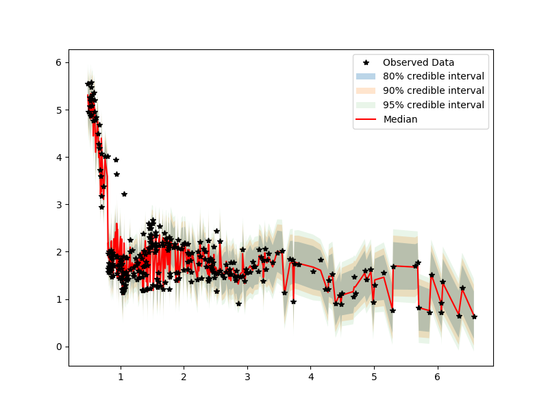
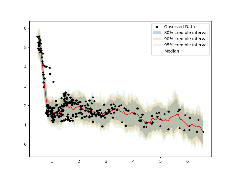 Posterior predictive: (10 samples)
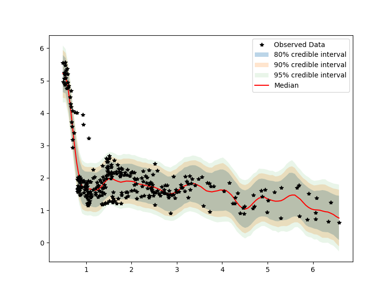
(100 samples)
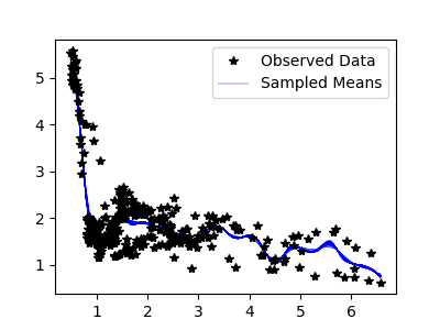
 Sampled means: (10 samples)

(100 samples)
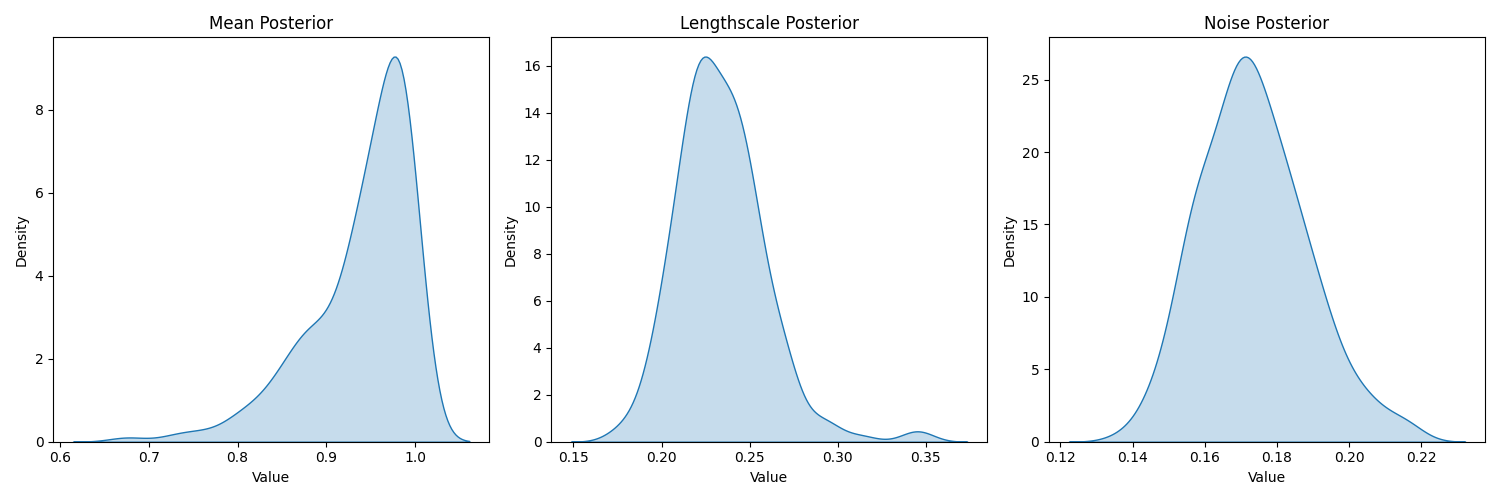
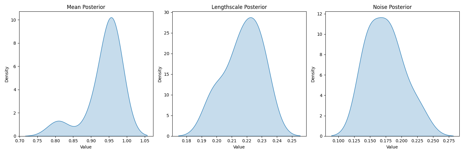 Posterior hyperparameters: (10 samples)
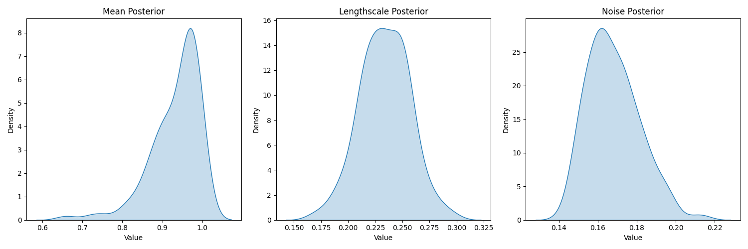
(100 samples)
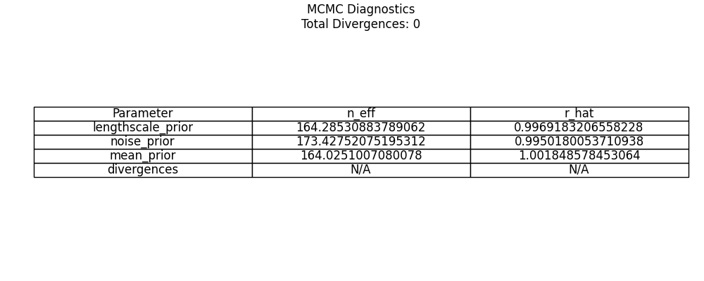
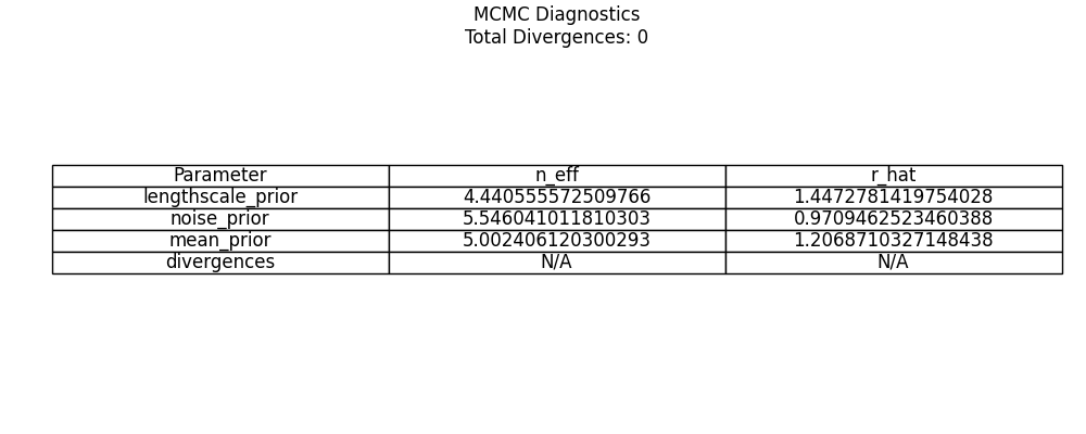 Diagnostics: (10 samples)
(100 samples)
Above, we can see that even with 100 samples we achieve healthy diagnostics for the rhats and number of efficient samples. Going one step further, we obtain results for 200 warm-up samples and 400 samples.

 Same plots, but with 600 samples
Increasing the samples, in this case, does very little (and it wasn’t needed).
Next, like in Model fits with supply shock, we can plot the GP now including supply shocks. Again, we use 100 warm-up samples and 100 samples.

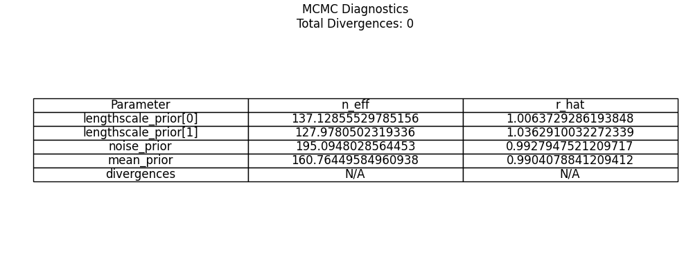
In this case, we can see that we might want to increase the samples, and perhaps increase the upper bound on the uniform prior range for the second lengthscale (one for each covariate, currently using the same prior specification). Technically, however, our R-hats are below 1.05, and we have healthy n_eff. Further, exploration with different priors and sample sizes provide nearly identical posterior predictive distributions.
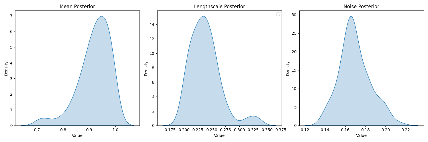
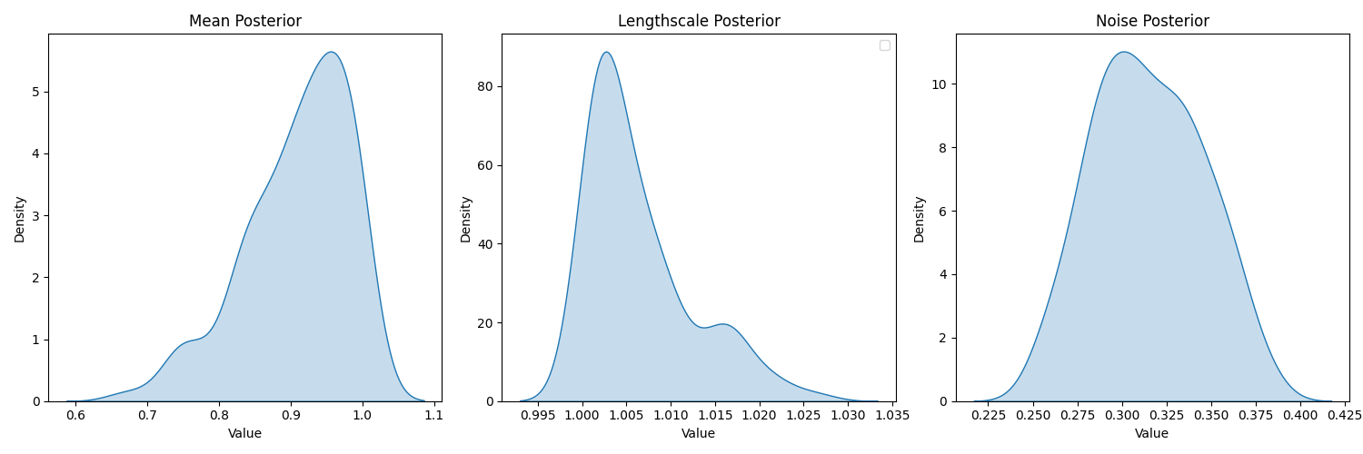
7.1 Examining hyperparameter priors


even with (0,100) prior we have posteriors
going overboard we have…
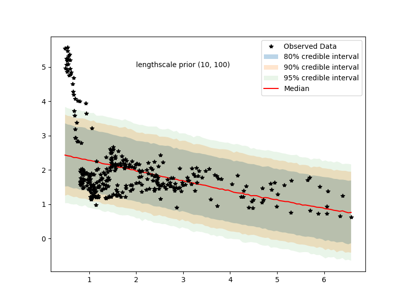
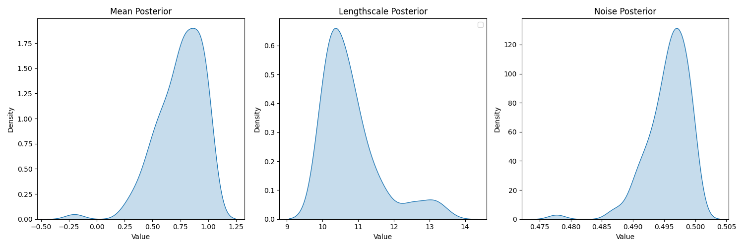
we see that lengthscale is heavily bent towards 10 (lower bound of prior for hyperparameter)
8 Modelling approach 4: (Bayesian) structural time varying vector autoregressive model
There are various schools of thought, but the reader might wonder whether or not the aggregate data is hiding relationships for different periods in time, or whether the data for “out-of-line” sub-periods is due to something else or random variation in the data. In turn, these sub-periods could be obscuring the “true” relationship between these two variables.
Roughly speaking, the above modelling approaches answer the question “if someone was told what unemployment (inflation) was at any point in time, then they would be able to respond with an answer regarding the value of inflation (unemployment) in turn. Then, if one is concerned with the joint path of inflation and unemployment through time, then we need another approach.
As a first step, let’s look at the joint evolution of these variables through the full period under question.
Modelling variables contemporaneously through time has often been associated with Structural Vector Autoregressive Models, a multivariate model of the contemporaneous variables (in this case inflation and unemployment). In these models, the covariates change through time, but the coefficients remain constant. However, we can go one step further and model changing covariates with changing coefficients by employing a Structureal Time Varying Vector Autoregressive model. For a basic discussion on identifiability and structural models, and how the the TV-VAR can take on a Dynamic Linear Model form, see the appendix.
While the above graph might be visually appealing, it is difficult to see if the structural time varying vector autoregressive model is doing no more than lagging a step or two behind the actual data. For this reason, we might want examine the plot below.
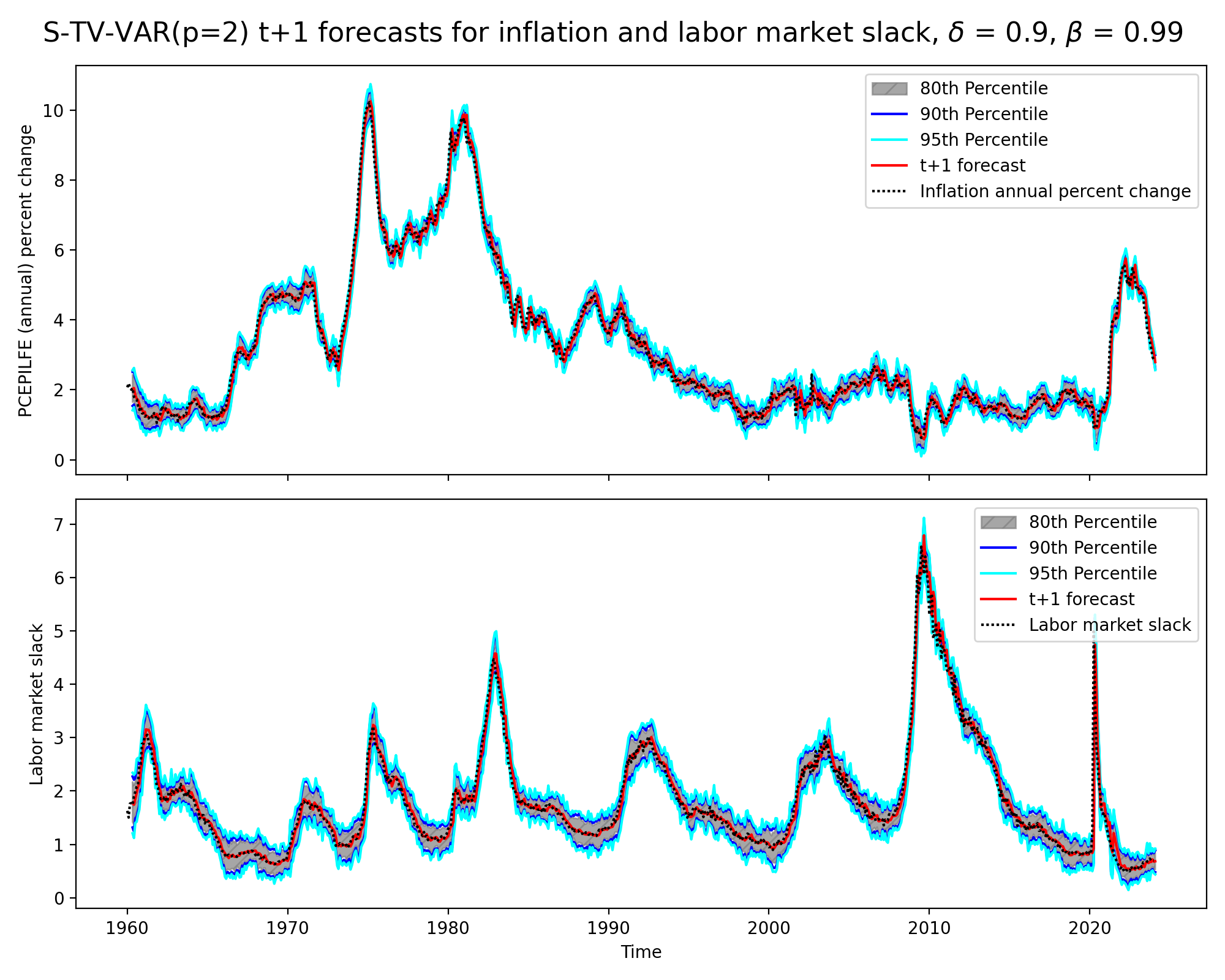
At first glance the model seems to forecast the data well. However, one should take into account that we are actually just seeing a strongly lagged effect (i.e., pick inflation next quarter to be inflation’s value last quarter). Rather, if the data changes drastically from quarter “a” to quarter “b” (e.g., around Covid), then the model is going to forecast quite poorly. For more gradual changes, the model will forecast better. Then, as a visual note, the graph contains nearly 770 time points, obscuring how far off the lagged forecasts are from the underlying data. The model above is using a state discount factor (\(\delta\)) of .9 and an observation discount of (\(\beta\)) of .99.
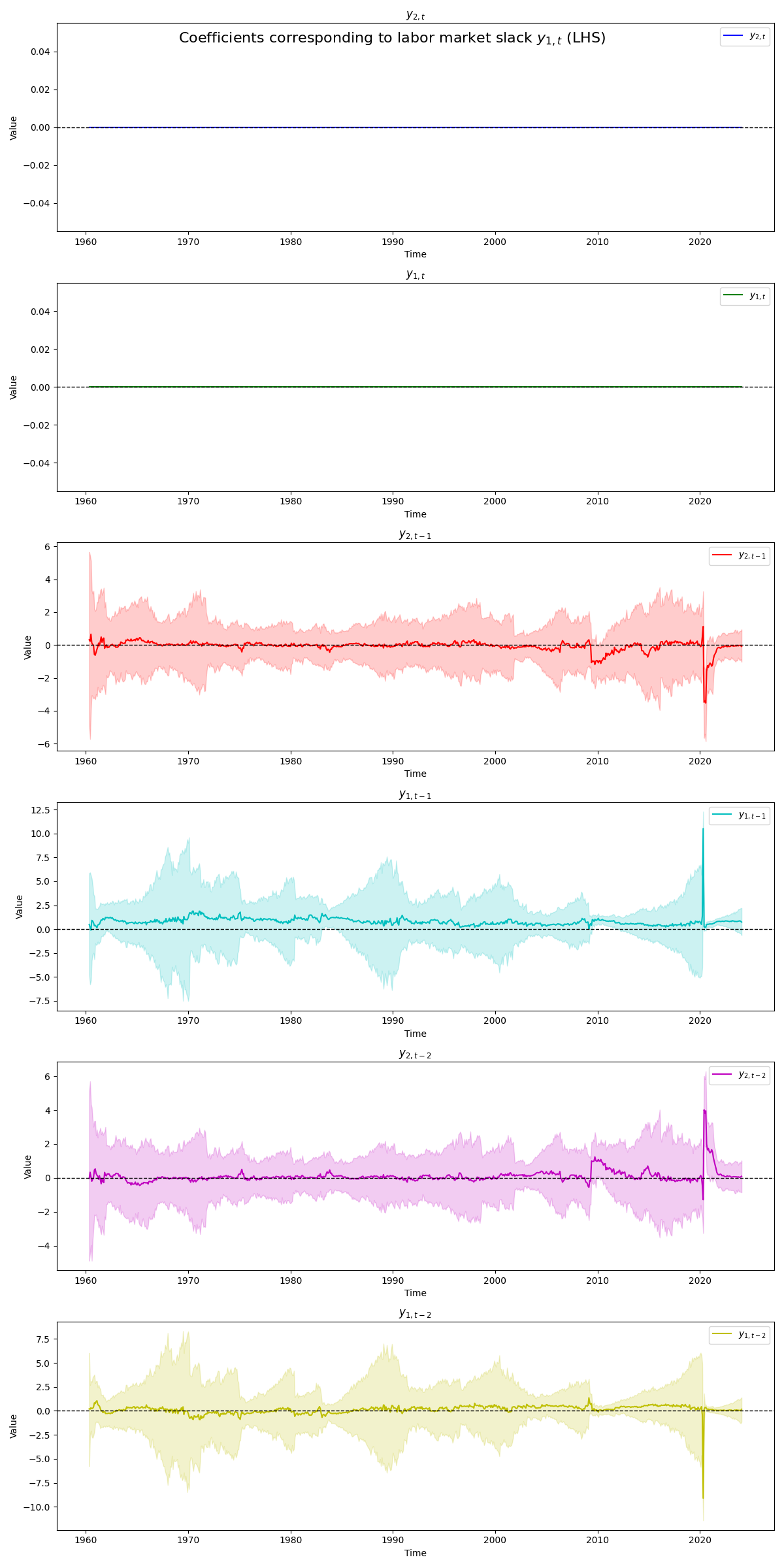
Finally, we can plot how the time-varying coefficients of the various lags used on the RHS of a series within our Structural TV-VAR(2). For this, we will just explore annual percent change in inflation for the LHS, and the implied corresponding lags used (see the appendix).
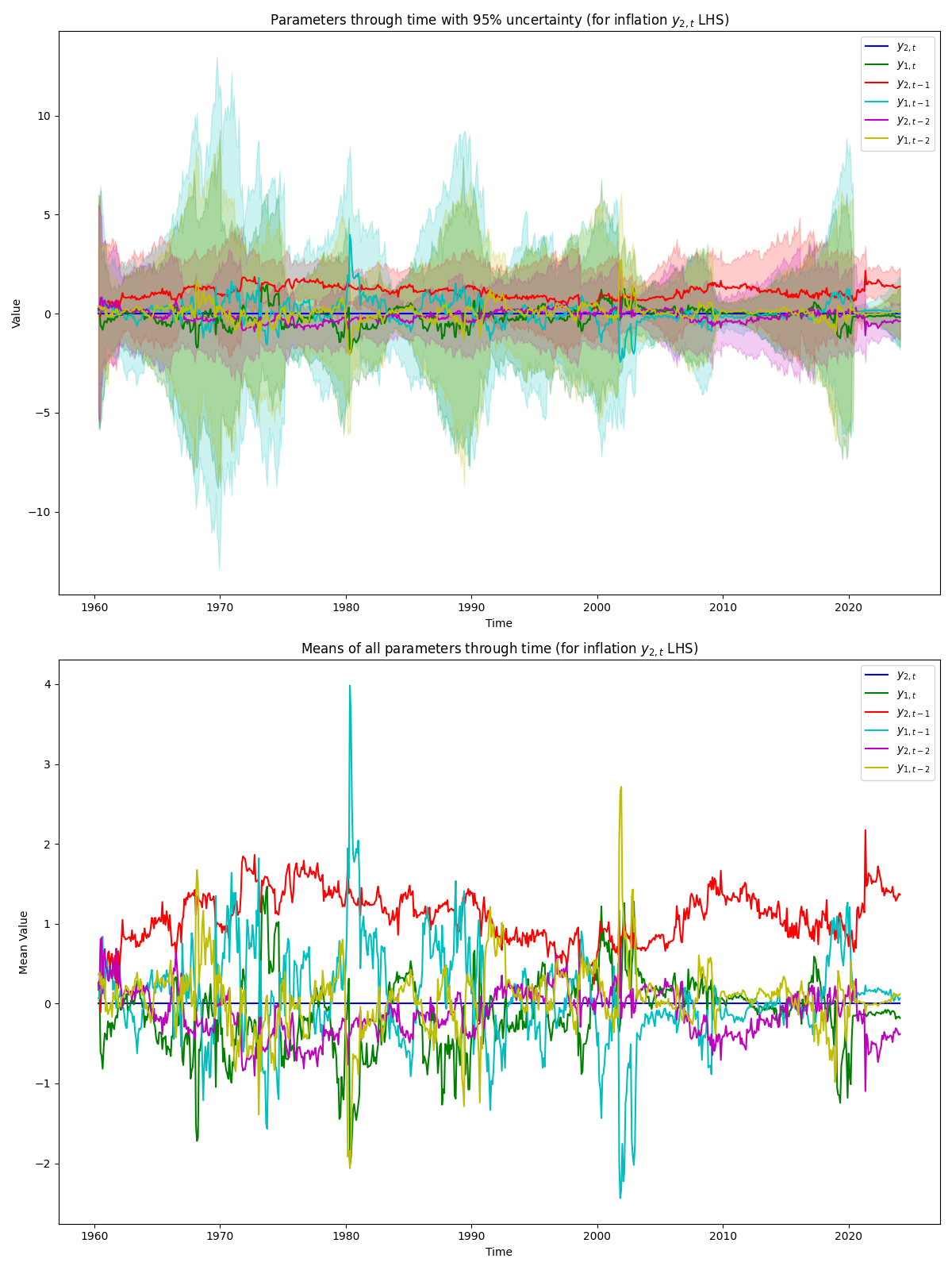
Here, we can see that the coefficient \(y_{2,t}\) is set to zero as described in the appendix. Then, and as likely expected given the forecast behavior seen above, we see the first lag \(y_{2,t-1}\) as playing the largest role throughout time. Overall, we see quite a lot of variation between the parameters throughout the full period. We see the contemporaneous labor market slack \(y_{1,t}\) negatively covary with the it’s other two lags throughout time (and with the first and second lag of inflation). Presumably, this is due to very high amount of multicolinearity between the different series and their lags. Then, similarly, we examine the coefficients of the covariates used for labor market slack \(y_{1,t}\) (LHS). Analogous statements to above can be made in this case. To see the coefficients in more detail see the subsequent side by side graph.

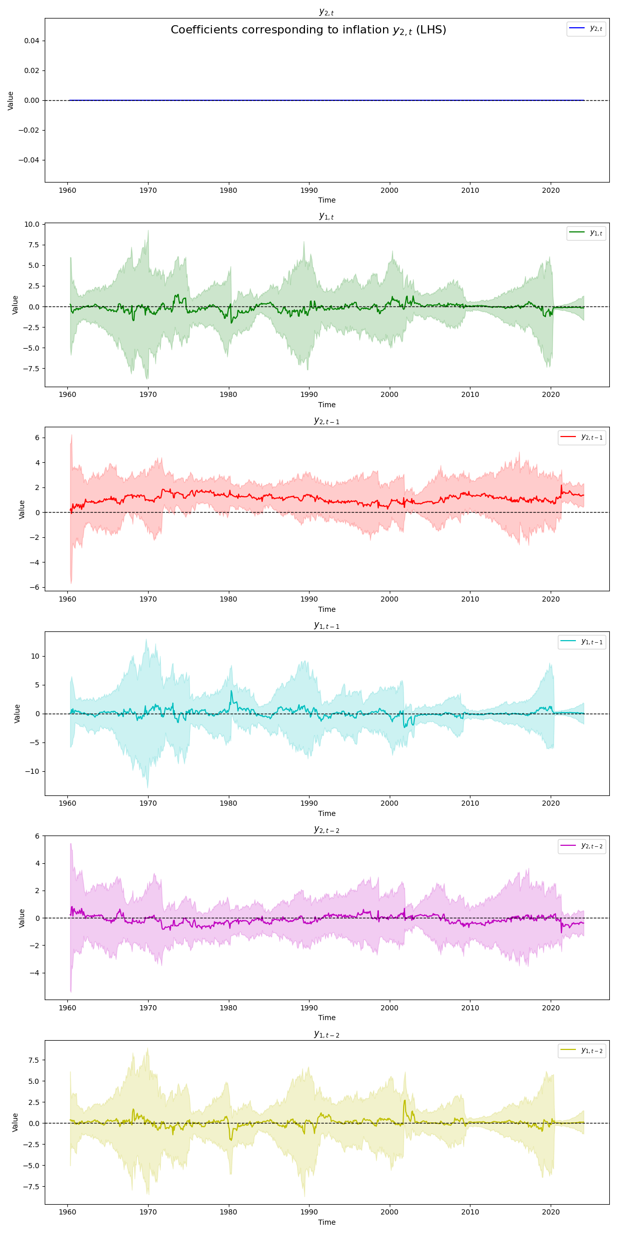
Below we can see that the \(y_{1,t}\) sets the first two coefficients to \(y_{2,t}\) and \(y_{1,t}\) to zero for identification purposes (“world order exclusion”). Then, below we see that \(y_{2,t-1}\) is the only coefficient that is consistently “not” zero, becoming significant at the 95% level at various points in time including very recent periods. Then, we can also see that the \(y_{1,t-1}\) is the only consistently not zero coefficient becoming significant at the 95% level at various periods. Then, we see a fairly tumultuous set of coefficient estimates corresponding to the LHS labor market slack series. Likely due to Covid, the model seems to drastically under and overweight coefficients (balancing each other out) before coming back to a relatively more stable recent period. Then, reading into the various periods where coefficients seem to pull away from zero for more consistent periods of time may deeper analysis, but one should generally keep in mind the effects of multicolinearity, lightly discussed above.
9 Paper
9.1 EDA (Paper?)
9.2 Rocket Ships (Paper)
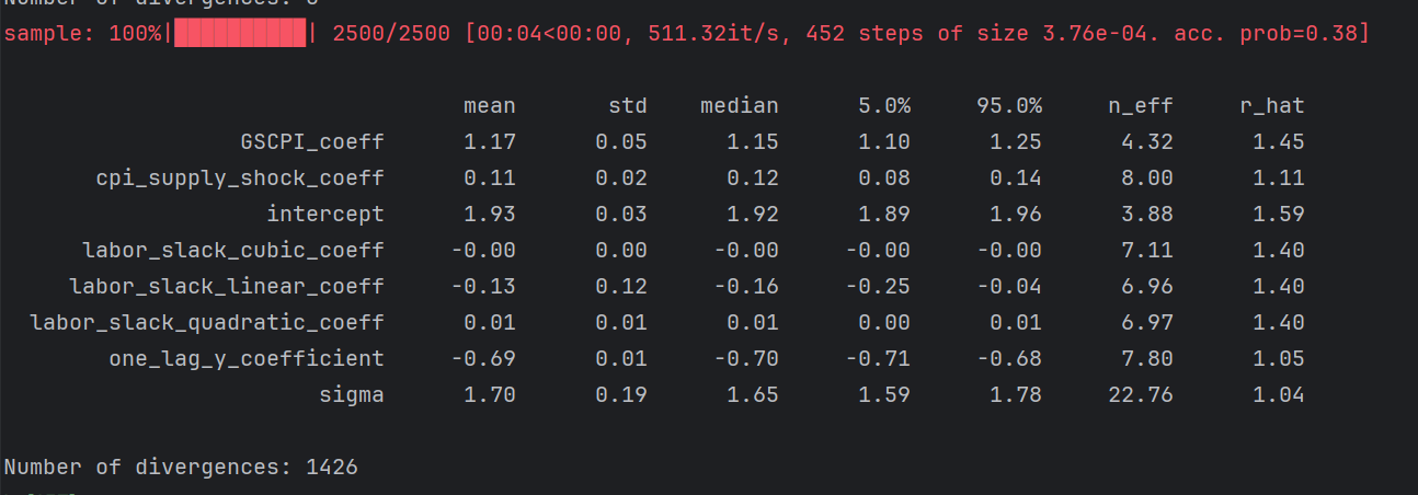
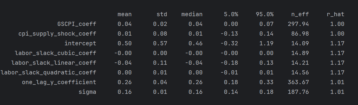
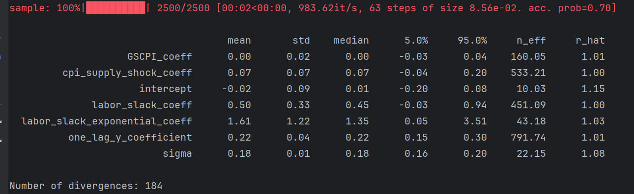
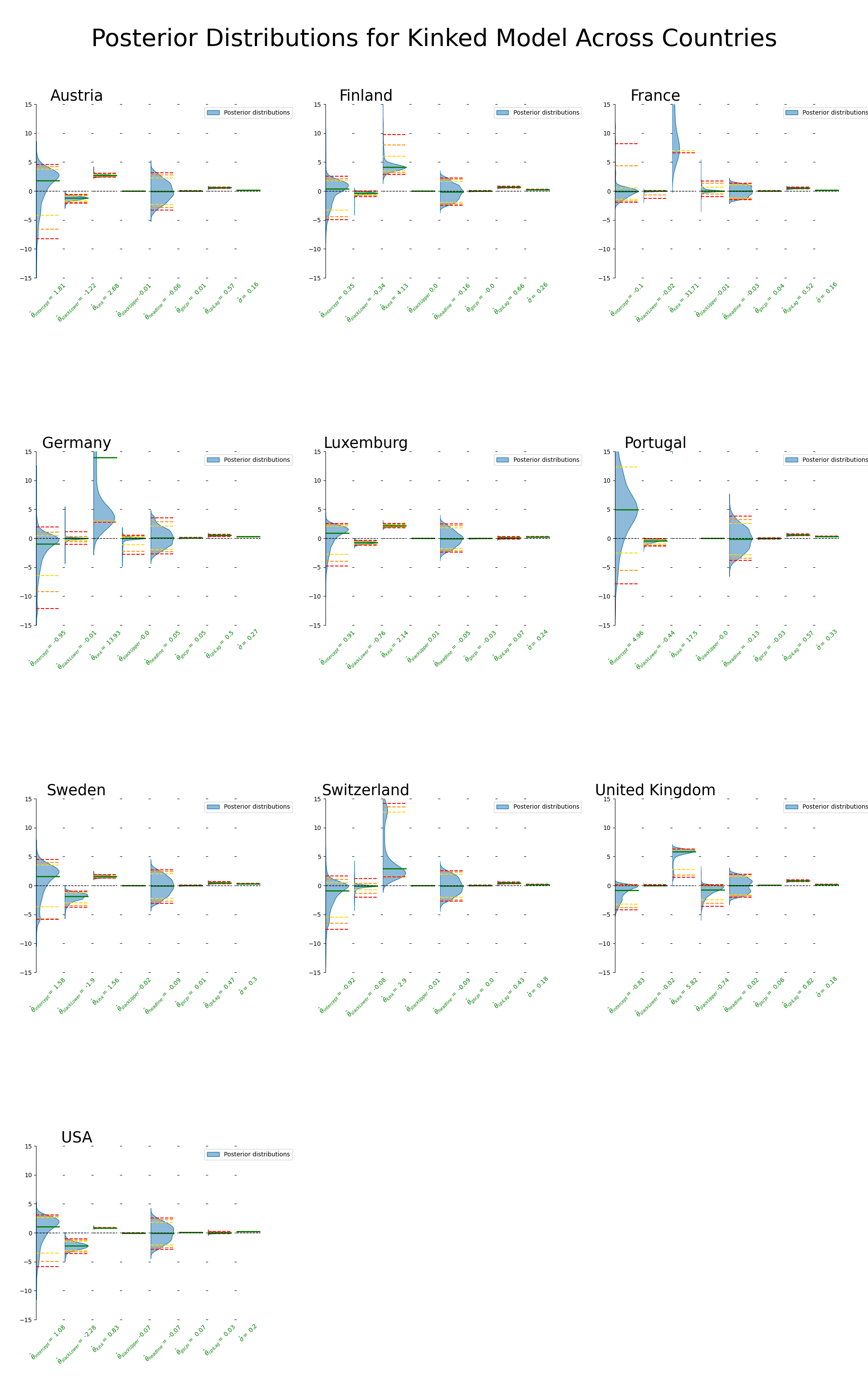
Titles, legends etc. can all be changed, this is just first draft for illustration. Also, I haven’t scrutinized everything yet. Note: the sampling needs to be examined as well - with all the new parameters, it’s not always fantastic sampling. Rhats seem to look fine, but the number of efficient samples can be far too low for various parameters for various countries. More to come.
9.2.1 Linear Across Countries
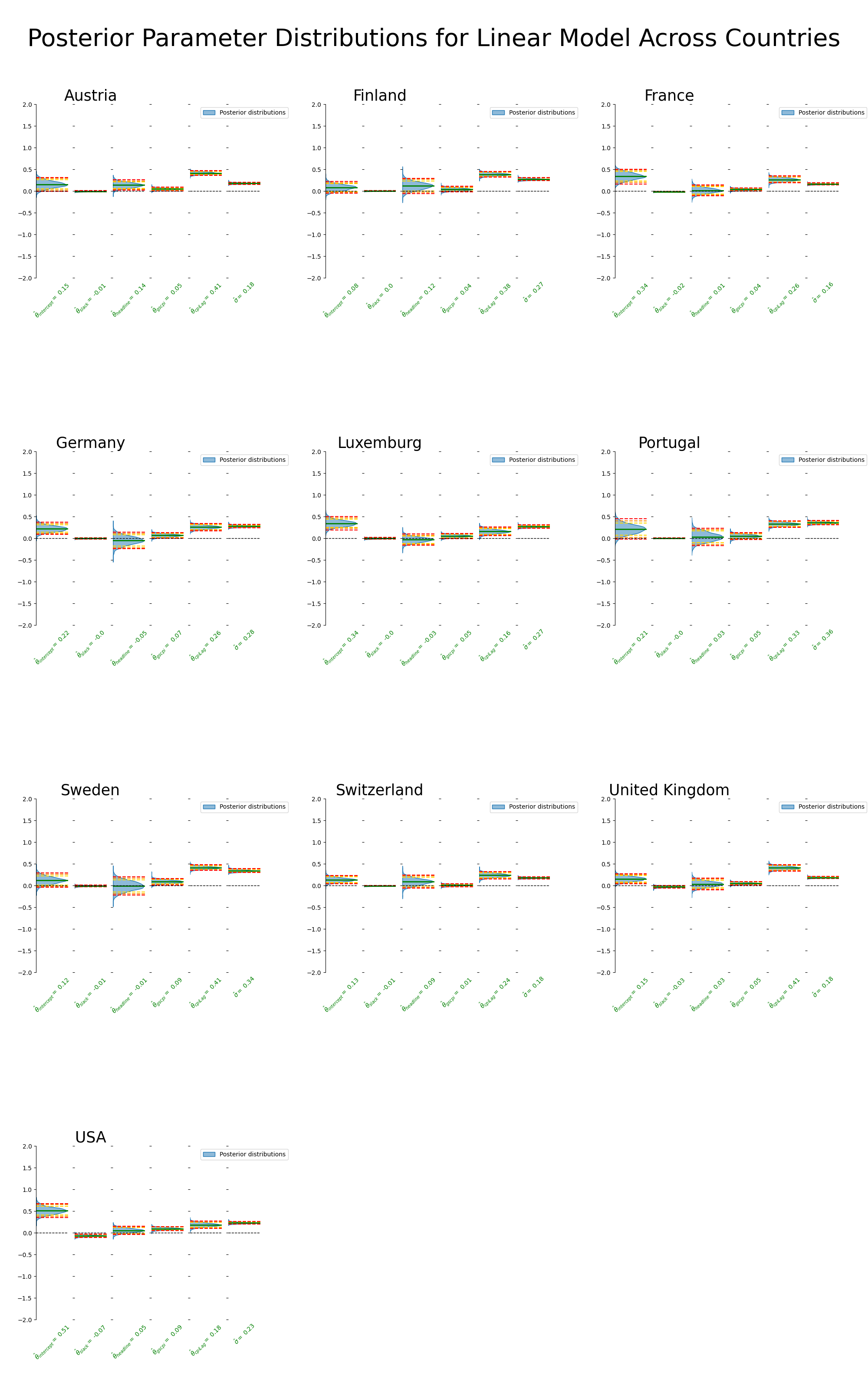
Sampling comments:
- everything healthy
9.2.2 Cubic Across Countries
Note that I change the scales slightly for the cubic y axis plots.
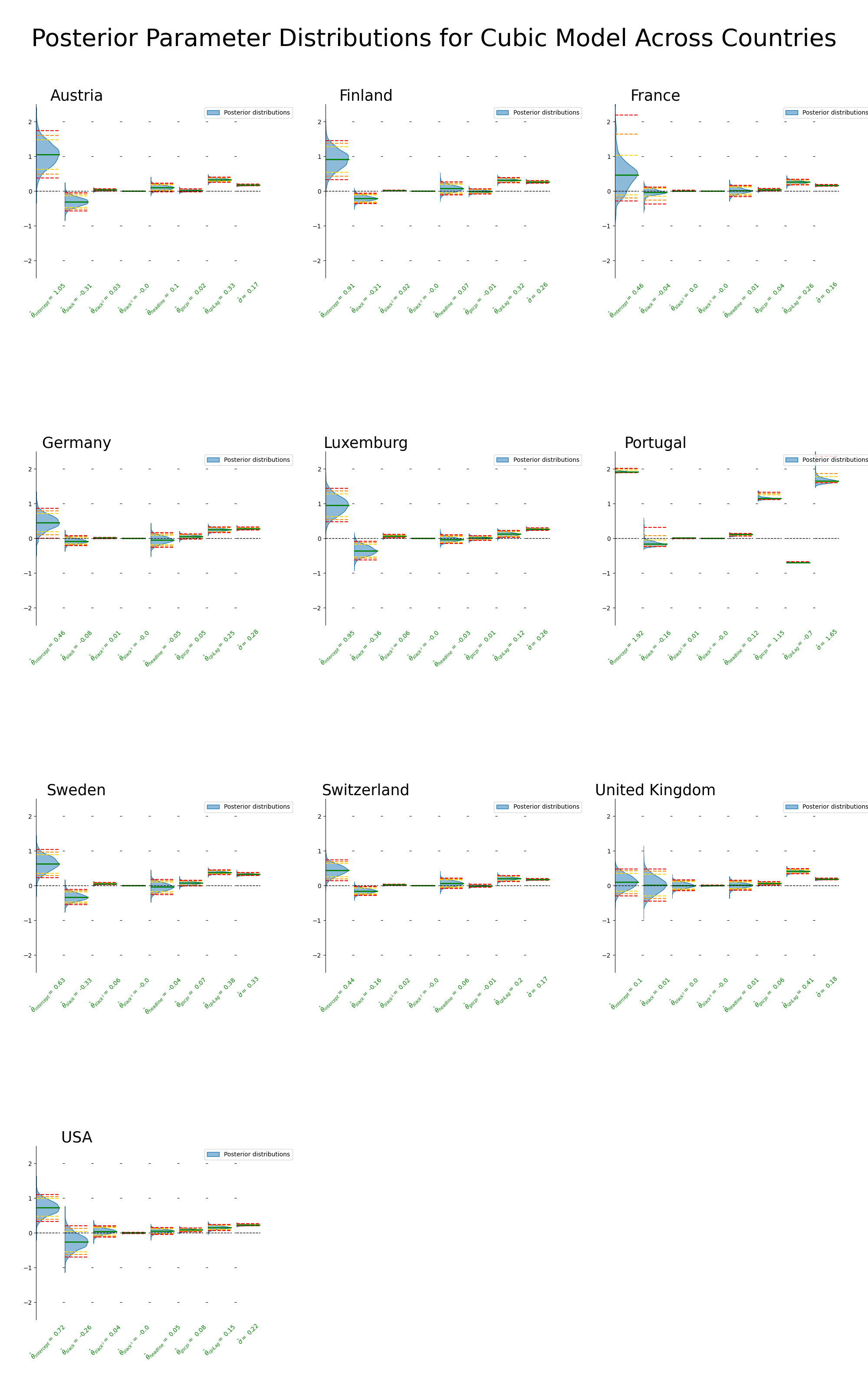
Sampling comments:
Portugal (red flag)
Self explanatory, all wrong, don’t trust Portugal results here
France
small n_eff for several and large rhats
Rest looks healthy
9.2.3 Exponential Across Countries
Notice I needed to change the y axis scale more so for the exponential case.
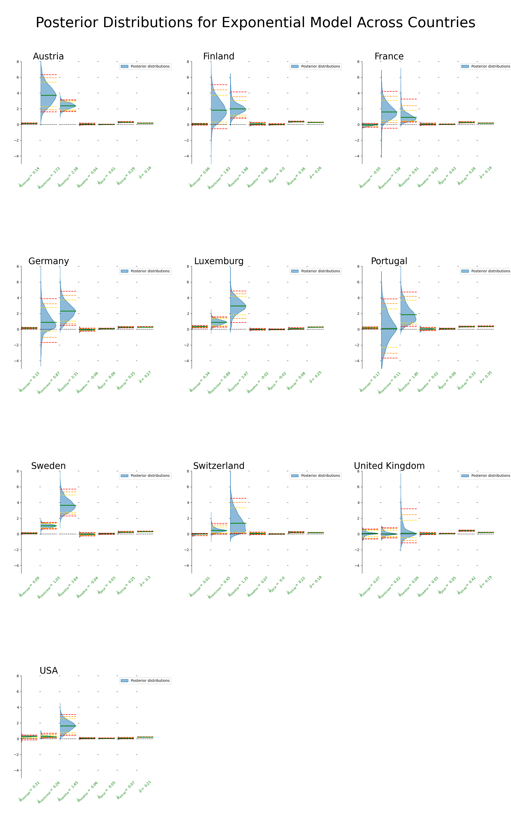
Sampling comments:
UK
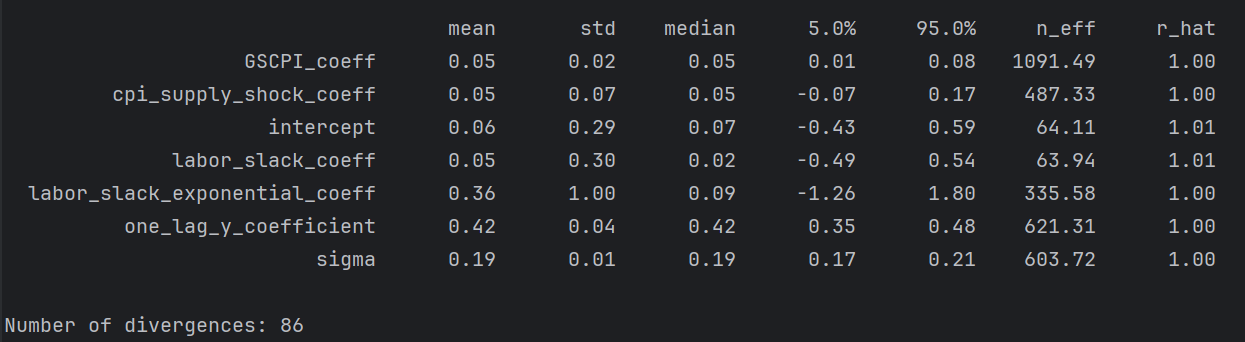
low n_eff for intercept and labor_slack_coeff
Switzerland
n_effs, rhats, and accept prob .7 (lower than desired)
Finland
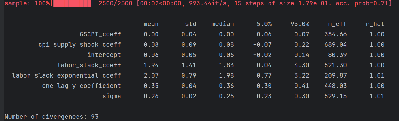
Intercept n_effs
Rest looks healthy
9.2.4 Kink Across Across Countries
Sampling comments:
France
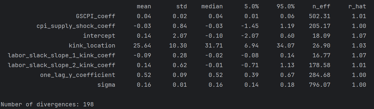
rhats and n_eff for intercept, kink_location, labor_slack_slope_1 (relatively more divergences)
UK
I’ve seen worse, small n_eff kink_location, second slope
Rest is healthy
10 Appendix
10.1 A: Kink Bayesian regression
The model is described below, along with a simulation.
10.1.1 Math:
The model is as follows where \(x\) is the unemployment rate and \(y\) is inflation
\[\begin{aligned} slope_1 &\sim N(0,2) \\ slope_2 &\sim N(0,2) \\ intercept_1 &\sim N(0,10) \\ kink_{location} &\sim Unif(min(x),\max(x))\\ \sigma &\sim exp(1)\\ intercept_2 &=intercept_1 + (slope_1 - slope_2)*kink_{location} \\ \mu(x) &= \begin{cases} \alpha_1 + \beta_1 x & \text{if } x < x_k \\ \alpha_2 + \beta_2 x & \text{if } x \geq x_k \end{cases} \\ \mathcal{L} &= \prod_{i}N(y_i|\mu(x_i),\sigma) \end{aligned}\]wherein posteriors are obtained via MCMC (HMC using the No-U-Turn Sampler).
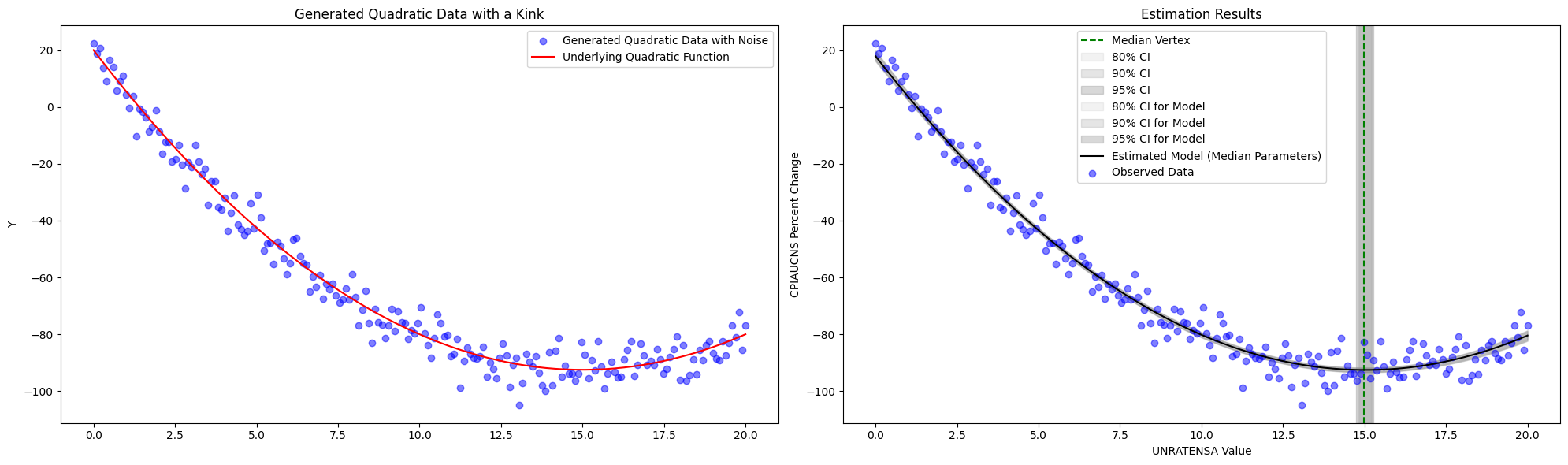
10.1.2 Simulation:
To see if the model is working as expected, we explore a few simulations. First we see the model succeed whether or not the generated data is convex or concave or if the kink location changes.
We do see limitations, however, in the subtly of the change in slope. With the specifications described above, we fit with \(slope_1 = -1.3\) and \(slope_2=-3.0\) with \(intercept_1 = 120\) and \(kink_{location}=75\) below, and we are still obtain the correct estimates. However, should the change slope become any more subtle, one should think about altering the priors slightly.
10.2 B: Bayesian Phillips (original) regression
The following results are using the model cited in (Benigno and Eggertsson 2023), where details are provided in the appendix. Roughly speaking, this model seems to behave more sensibly than either the quadratic or cubic models. Similarly, we take the original Phillips model and turn it Bayesian
\[\begin{aligned} a & \sim N(0,2) \\ b & \sim N(0,2) \\ c & \sim N(0,2) \\ \sigma &\sim exp(1) \\ \mu(x) &= a + b(\frac{1}{x})^{c} \\ y & \sim N(\mu(x),\sigma) \end{aligned}\]
10.3 C: Bayesian Phillips (linear model)
10.4 D: Quadratic Bayesian regression
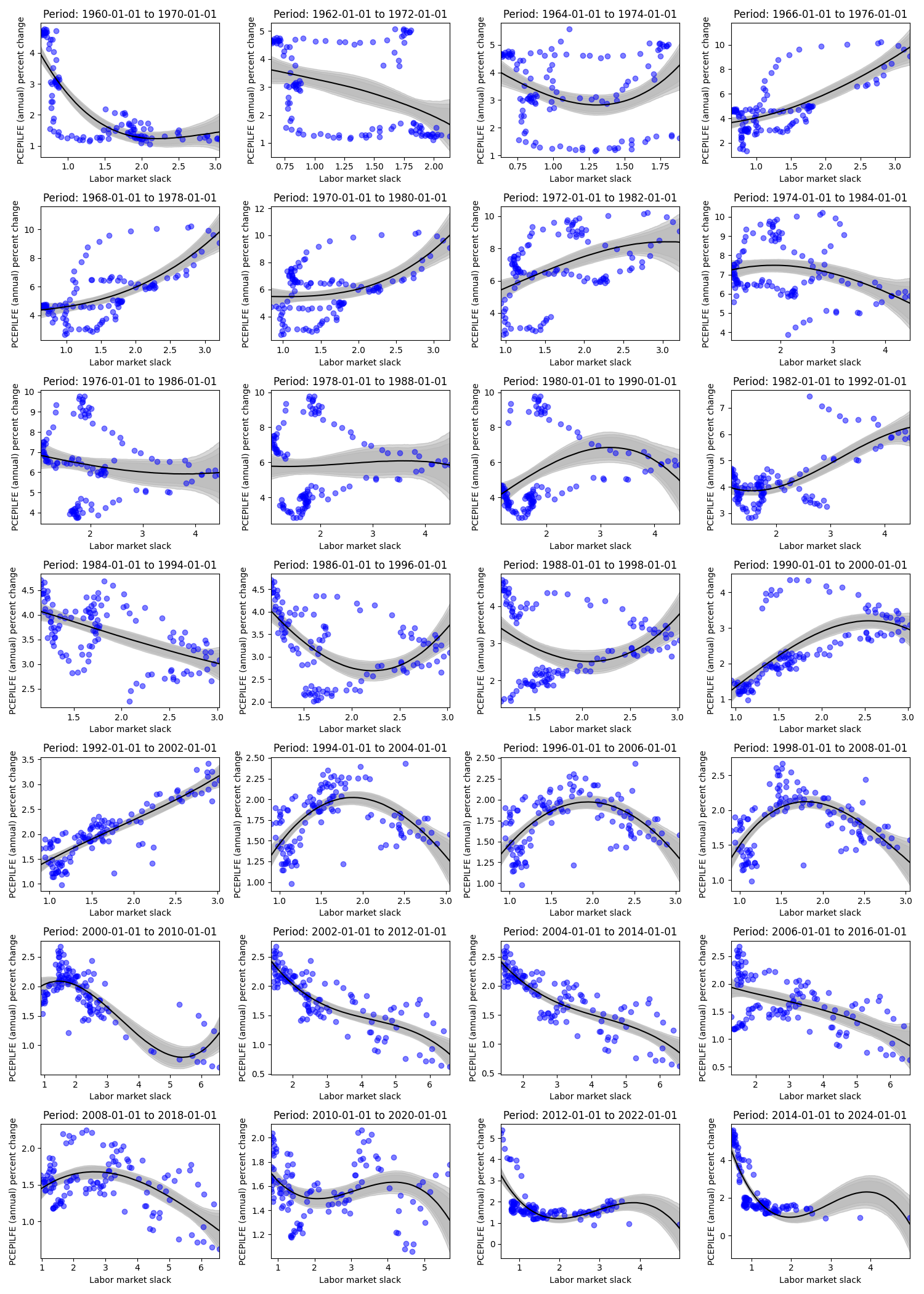
Again let’s examine the full period’s data below. Note that the vertex is included with uncertainty intervals.
And, again let’s examine 10 year’s worth of data every year
Above, our model is quadratic, and so by construction, there is an emphasis on the model having both positive and negative slopes (i.e. parabolic). Clearly these parametric assumptions play a heavy hand in many cases. However, it may fit the data slightly better for the periods 1994-2004, 1996-2006, and 1998 to 2008 where the data does indeed show a parabolic scatter plot. Thresholds, analogous to above, are shown below.
Essentially, the quadratic model is incapable of discovering the kink due to its over-powering parametric assumptions.
The model for the Quadratic Bayesian Regresion model is straightfoward
10.4.1 Math:
\[\begin{aligned} a & \sim \mathcal{N}(0,2) \\ b & \sim \mathcal{N}(0,2) \\ c & \sim \mathcal{N}(0,10) \\ \sigma & \sim \operatorname{Exponential}(1) \\ \mu(x) & =a x+b x^2+c \\ y & \sim \mathcal{N}(\mu(x), \sigma) \end{aligned}\]10.4.2 Simulation:

A note on the estimation of the vertices. The above simply takes the posterior samples to calculate the vertices, e.g., \(vertex^{(s)} = x^{(s)} = -\frac{a^{(s)}}{2b^{(s)}}\), and so we take the median of these samples \((s)\) from the posterior samples of \(a\) and \(b\). Similarly we get percentiles.
10.5 E: Cubic Bayesian regression
Keeping in mind the problematic upward sloping curve on the right hand side of many graphs due to the parabolic nature of the quadratic graph, we can alter the model to include a cubic term. Vertices are omitted in this portion.
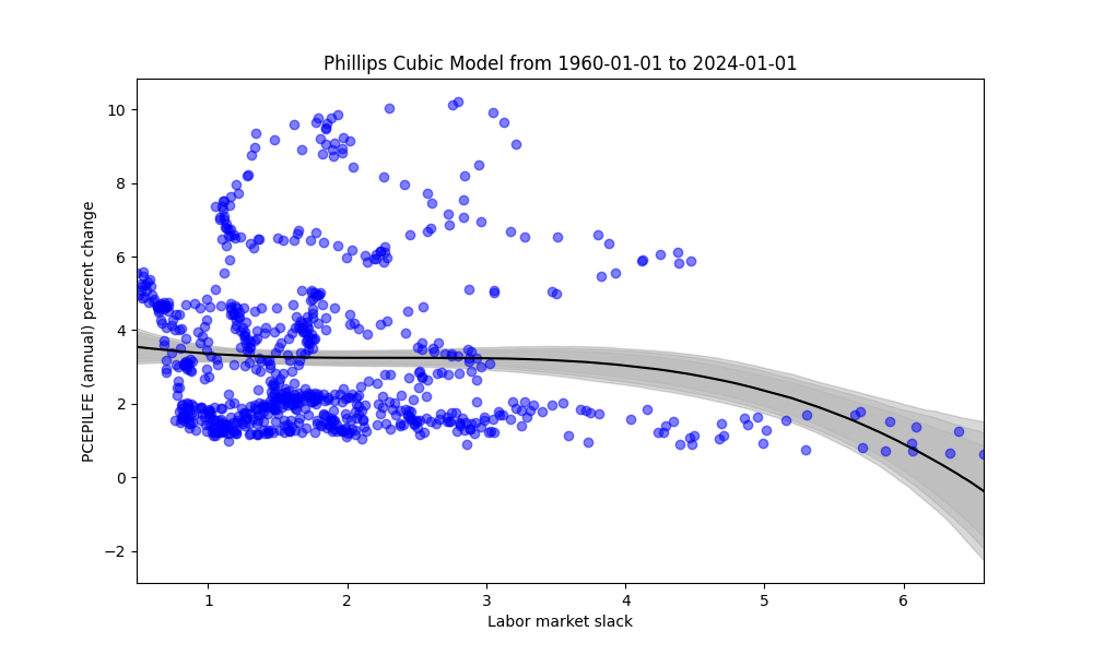 In general, these models look more reasonable than the quadratic model. However, we can see that there is a forced polynomial (cubic) behavior, particularly if there is little data at the higher range of labor market slack values.
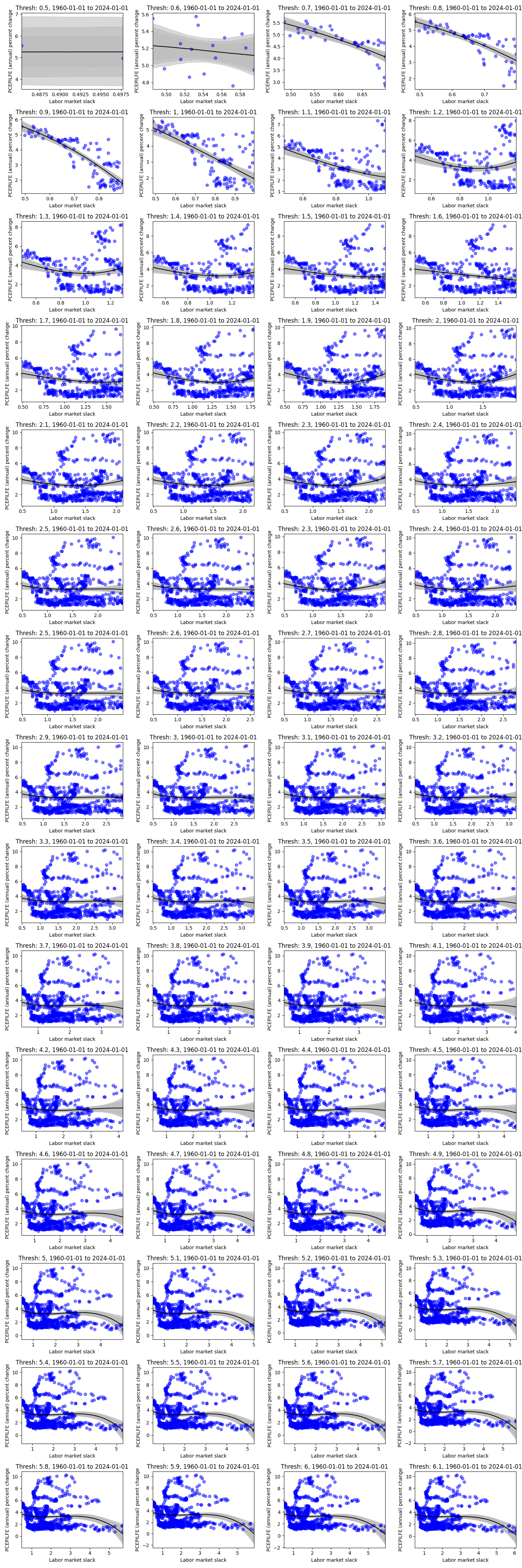
Similarly, we can explore the thresholds. Similar to the quadratic model, the cubic model struggles to distinctively display the “kink” due to its parametric (polynomial) structure.
The model is as follows,
\[\begin{aligned} a & \sim \mathcal{N}(0,2) \\ b & \sim \mathcal{N}(0,2) \\ d & \sim \mathcal{N}(0,2) \\ c & \sim \mathcal{N}(0,10) \\ \sigma & \sim \operatorname{Exponential}(1) \\ \mu(x) & =ax + bx^2 + dx^3 + c \\ y & \sim \mathcal{N}(\mu(x), \sigma) \end{aligned}\]Simulations omitted.
10.6 F: Bayesian structural time varying vector autoregressive (S-TV-VAR(p))
A few notes on identification and model construction are discussed below.
10.6.1 Identification:
As a first pass, one might attempt to the two series contemporaneously in the following manner
\[\begin{aligned} y_{1t} &= -b_{12}y_{2t} + \gamma_{11}y_{1,t-1} + \gamma_{12}y_{2,t-1} + \varepsilon_{1t} \\ y_{2t}&=-b_{21}y_{1t} + \gamma_{21}y_{1,t-1} + \gamma_{22}y_{2,t-1} + \varepsilon_{2t} \end{aligned}\]
where
\[\boldsymbol{\varepsilon}_t \overbrace{\sim}^{iid} N\left(\mathbf{0},\begin{pmatrix} \sigma_{1}^{2} & 0 \\ 0 & \sigma_{2}^2 \end{pmatrix} \right)\]
but, we can typically not make the statement \(\mathbb{C}(y_{2t},\varepsilon_{1t}) \neq 0\) modelling all variables in an endogenous manner like above.
Note that we can rewrite above in the form
\[\mathbf{B}\mathbf{y}_t = \Gamma \mathbf{y}_{t-1} + \varepsilon_{t}\]
and in “reduced form” as
\[\mathbf{y}_t = \mathbf{A}\mathbf{y}_{t-1} + \mathbf{u}_t\].
Then, note that in doing so we have
\[\begin{aligned} \mathbf{A} &= \mathbf{B}^{-1}\boldsymbol{\gamma} \\ \boldsymbol{\Omega} = \mathbb{V}(\mathbf{u}_t) &= \mathbb{V}[\mathbf{B}^{-1}\boldsymbol{\varepsilon}_t] = \mathbf{B}^{-1}\mathbf{D}\mathbf{B^{-1}}' \end{aligned}\]
and, we find that the reduced form (left) as one less parameter than the structural form (right), meaning it is not possible to uniquely travel between the the two forms. However, we can implement a restriction such that the “first” series in the multivariate model is no longer a function of the “second” series. This is equivalent to setting a constraint that one of the parameters in the structural form is set to zero, allowing for unique solutions. This is sometimes referred to as “world ordering”. The above referenced example, and more notes are found here.
10.6.2 Dynamic linear model formulation:
The modelling construction in this analysis uses a Dynamic Linear Model. As is often the case for many time series models, one can rewrite the TV-VAR(p) in a Dynamic Linear Model. Then, through “world ordering” we can jump from a TV-VAR(p) to a Structural TV-VAR(p).
One can write a TV-VAR(p) as
\[\underbrace{\mathbf{y}_t}_{q\times1} = \sum_{1:p}\underbrace{\boldsymbol{\Phi}_{t,r}}_{q\times q}\mathbf{y}_{t-r} + \boldsymbol{\nu}_t\]
where \(\boldsymbol{\nu}_t \sim N(\mathbf{0},\underbrace{\mathbf{V_t}}_{q\times q})\). However, we can also reformulate the model as a Dynamic Linear Model
\[\underbrace{\mathbf{y}_t}_{q \times 1} = \underbrace{\boldsymbol{\Theta}_t}_{[q\times (p+1)q]} \underbrace{\mathbf{F}_t}_{(p+1)q \times 1} + \boldsymbol{\nu}_t\]
where
\[ \begin{aligned} \mathbf{y}_t &=\begin{pmatrix} \left(\boldsymbol{\theta}_{t,1}^{(2)'}\right)_{1 \times q},& \ldots &,\left(\boldsymbol{\theta}_{t,p}^{(2)'}\right)_{1 \times q} \\ \left(\boldsymbol{\theta}_{t,1}^{(1)'}\right)_{1 \times q},&\ldots &,\left(\boldsymbol{\theta}_{t,p}^{(1)'}\right)_{1 \times q}\end{pmatrix}\begin{pmatrix}\mathbf{y}_{t-1}\\\vdots\\\mathbf{y}_{t-p-1}\end{pmatrix} + \boldsymbol{\nu}_t \end{aligned} \]
Where \(q = 2\), and where \((1), (2)\) refers to coefficients associated with the first and second series in \(\mathbf{y}_t\), respectively. Or, we have
\[\left(\boldsymbol{\theta}_{t,1}^{(2)'} \right) = (\theta_{t,1,2}^{(2)},\theta_{t,1,1}^{(2)})\]
where the third subscript denotes which covariate is being hit. For example
\[(\theta_{t,1,2}^{(2)},\theta_{t,1,1}^{(2)})\mathbf{y}_{t-1} = \theta_{t,1,2}^{(2)}y_{2,t-1} + \theta_{t,1,1}^{(2)}y_{1,t-1}\].
Finally, let’s convert this to a structural formulation.
\[ \begin{aligned} \mathbf{y}_t &=\begin{pmatrix} \left(\boldsymbol{\theta}_{t,1}^{(2)'}\right)_{1 \times q},& \ldots &,\left(\boldsymbol{\theta}_{t,p+1}^{(2)'}\right)_{1 \times q} \\ \left(\boldsymbol{\theta}_{t,1}^{(1)'}\right)_{1 \times q},&\ldots &,\left(\boldsymbol{\theta}_{t,p+1}^{(1)'}\right)_{1 \times q}\end{pmatrix}\begin{pmatrix}\mathbf{y}_{t}\\\vdots\\\mathbf{y}_{t-p}\end{pmatrix} + \boldsymbol{\nu}_t \end{aligned} \]
where we have
\[\begin{pmatrix}y_{2t} \\ y_{1t} \end{pmatrix} = \begin{pmatrix} \theta_{t,1,2}^{(2)},\theta_{t,1,1}^{(2)},\theta_{t,2,2}^{(2)},\theta_{t,2,1}^{(2)},\ldots,\theta_{t,p+1,2}^{(2)},\theta_{t,p+1,1}^{(2)} \\ \theta_{t,1,2}^{(1)},\theta_{t,1,1}^{(1)},\theta_{t,2,2}^{(1)},\theta_{t,2,1}^{(1)},\ldots,\theta_{t,p+1,2}^{(1)},\theta_{t,p+1,1}^{(1)} \end{pmatrix}\begin{pmatrix} y_{2,t}\\y_{1t} \\y_{2,t-1} \\y_{1,t-1} \\ \vdots \\ y_{2,t-p} \\ y_{1,t-p}\end{pmatrix} + \boldsymbol{\nu}_t\]
but note that we need to set \(\theta_{t,1,2}^{(2)} = \theta_{t,1,1}^{(1)} = 0\) since we don’t allow for \(y_{2t} = \theta_{t,1,2}^{(2)}y_{2t} + \ldots\) nor \(y_{1t} = \theta_{t,1,1}^{(1)}y_{1t} + \ldots\). Then, to obtain identification through an ordering exclusion constraint, we set \(\theta_{t,1,2}^{(1)}=0\) so that \(y_{1t}\) does not include \(y_{2t}\) in the right hand side. Rather the ordering starts with \(y_{1t}\). Note that we have \(p+1\) coefficients for each series on the LHS since we include \(p\) lags for each of the contributing series on the corresponding RHS, and their contemporaneous coefficients.
Then, one notes that a Structural TV-VAR(p) is in a flexible Dynamic Linear Model where one can now place a random walk on the time varying matrix of coefficients. In this exchangeable time series multivariate DLM setting, one can incorporate cross-sectional covariation, not just at the observation level, but a the state level as well. In matrix notation we have
\[\begin{aligned}\underbrace{\mathbf{y}_t}_{q \times 1} &= \underbrace{\boldsymbol{\Theta}_t}_{[q\times (p+1)q]} \underbrace{\mathbf{F}_t}_{(p+1)q \times 1} + \boldsymbol{\nu}_t, \qquad\boldsymbol{\nu}_t \sim N(\mathbf{0},\mathbf{V}_t) \\ \boldsymbol{\Theta}_t &=\boldsymbol{\Theta}_{t-1} + \boldsymbol{\Omega}_t, \qquad\qquad \qquad\boldsymbol{\Omega}_t \sim N(\mathbf{0},\mathbf{W}_t, \mathbf{V_t}) \end{aligned}\]
where \(\mathbb{C}(\nu_{t,i},\nu_{t,j})=v_{t,i,j}\) and \(\mathbb{C}(\boldsymbol{\omega}_{t,i},\boldsymbol{\omega}_{t,j})=v_{t,i,j}\mathbf{W}_t\) and we can equivalently write the above as
\[\begin{aligned} y_{t,j} &= \boldsymbol{\theta}^{(j)}_t\mathbf{F}_t + \nu_{t,j}, \qquad\nu_{t,j} \sim N(0,v_{t,j,j}) \\ \boldsymbol{\theta}^{(j)}_t &=\boldsymbol{\theta}^{(j)}_{t-1} + \boldsymbol{\omega}_{t,j}, \qquad\boldsymbol{\omega}_{t,j}\sim N(\mathbf{0},v_{t,j,j}\mathbf{W}_t) \end{aligned}\]
However, in our case we simply use state discounting with no use of cross-sectional covariation at the state level. One difficult aspect of this model is the sheer quantity of parameters as the number of lags (\(p\)) and number of series (\(q\)) grow.* With these specifications we can choose to keep known, and possibly constant, covariance matrices through time, use unknown covariance matrices through time (by using a conjugate InverseWishart prior), or incorporate discounting through a Matrix-Beta random walk on the InverseWishart distributed observation covariance matrix. In the analysis above, the choice is to use the Matrix-Beta random walk on the unknown InverseWishart distributed observation covariance, and to use standard state covariance discounting. For more on Dynamic Linear Models and TV-VARs, see [West and Harrison (1997)](Prado, Ferreira, and West 2021).
*For structural approaches that incorporate sparsity, see the Dynamic Dependency Network Model (DDNM) (Zhao, Xie, and West 2016), or the extension to the Simultaneous Graphical Dynamic Linear Model (SGDLM) (Gruber and West 2017) which no longer suffers from “ordering” constraints.
10.7 G: Gaussian Process Math (priors on hyperparameters + HMC)
\[\begin{aligned} y&=f(x \mid \boldsymbol{\theta})+\epsilon\\ \epsilon &\sim N(0,\sigma^2)\\ f(x|\boldsymbol{\theta}) &\sim \mathcal{GP}(\mu(x|\boldsymbol{\theta}),k(x,x'|\boldsymbol{\theta}))\\ k(x,x') &=exp\left(\frac{||x-x'||^2}{2l^2}\right)\\ \sigma^2 &\sim Unif(.01,.5) \\ l^2 &\sim Unif(.01,.5) \\ \mu(x|\boldsymbol{\theta}) &\sim Unif(-1,1) \end{aligned} \]
More coming…